Survival Analysis Step 3.0: Mediation Analysis

What this step is for

This tutorial is the Step 3.0 survival-analysis article in leo.ukb. After a main Cox model and any subgroup or interaction work, a different question may arise:

does part of the exposure-outcome association operate through a mediator?

That is a mediation question, not a subgroup question and not an interaction question.

First separate mediation from interaction

The current survival-analysis workflow in leo.ukb answers three different questions:

Step 1: is there a main exposure-outcome association?
Step 2: does that association differ across groups, and on which scale?
Step 3.0: is part of that association transmitted through a mediator?

This distinction matters because:

interaction is about effect heterogeneity
mediation is about a pathway decomposition

In other words, mediation does not replace Step 1 or Step 2. It builds on them.

Start from the data and analytic roles

We use a synthetic example with a rare event, a binary exposure, a binary mediator, and several covariates.

set.seed(20260323)
n <- 500
age <- rnorm(n, 60, 8)
bmi <- rnorm(n, 26, 4)
smoking <- factor(sample(c("Never", "Ever"), n, replace = TRUE))
exposure_num <- rbinom(n, 1, plogis(-0.2 + 0.02 * (age - 60)))
mediator_num <- rbinom(n, 1, plogis(-0.5 + 0.9 * exposure_num + 0.02 * (bmi - 26)))
hazard_rate <- exp(
  -5.8 + 0.55 * exposure_num + 0.40 * mediator_num +
    0.02 * (age - 60) + 0.03 * (bmi - 26) + 0.20 * (smoking == "Ever")
)
event_time <- rexp(n, rate = hazard_rate)
censor_time <- rexp(n, rate = 0.08)

med_df <- data.frame(
  outcome = as.integer(event_time <= censor_time),
  outcome_censor = pmax(pmin(event_time, censor_time), 0.2),
  exposure = factor(exposure_num, levels = c(0, 1), labels = c("Low risk", "High risk")),
  mediator = factor(
    mediator_num,
    levels = c(0, 1),
    labels = c("Low inflammation", "High inflammation")
  ),
  age = age,
  bmi = bmi,
  smoking = smoking
)

Before fitting anything, look at the analytic roles explicitly.

dplyr::glimpse(med_df)
#> Rows: 500
#> Columns: 7
#> $ outcome        <int> 0, 0, 0, 0, 0, 0, 0, 0, 0, 0, 0, 0, 1, 1, 0, 0, 0, 0, 0…
#> $ outcome_censor <dbl> 2.6117515, 6.4186284, 8.6449270, 5.6413310, 12.1900483,…
#> $ exposure       <fct> High risk, High risk, Low risk, High risk, Low risk, Lo…
#> $ mediator       <fct> Low inflammation, High inflammation, Low inflammation, …
#> $ age            <dbl> 59.73588, 59.19772, 45.83227, 57.49797, 46.83760, 55.76…
#> $ bmi            <dbl> 27.17832, 27.91178, 30.48299, 24.70933, 22.63096, 28.43…
#> $ smoking        <fct> Never, Never, Never, Never, Never, Ever, Ever, Ever, Ev…

Analytic roles in the Step 3 teaching data frame
Variable	Type	Step 3 role
`outcome`	Binary event indicator	Incident outcome event
`outcome_censor`	Follow-up time	Incident outcome follow-up time
`exposure`	Binary exposure	Exposure to be decomposed
`mediator`	Binary mediator	Candidate pathway variable
`age`	Continuous covariate	Adjustment covariate
`bmi`	Continuous covariate	Adjustment covariate
`smoking`	Binary covariate	Example covariate that requires explicit `x_cov_cond`

Inspect the analysis-ready data before fitting

As in Step 1 and Step 2, it helps to inspect the analysis-ready cohort before moving to the model.

knitr::kable(utils::head(med_df, 6))

outcome_censor	exposure	mediator	age	bmi	smoking
2.611752	High risk	Low inflammation	59.73588	27.17832	Never
6.418628	High risk	High inflammation	59.19772	27.91178	Never
8.644927	Low risk	Low inflammation	45.83227	30.48299	Never
5.641331	High risk	Low inflammation	57.49797	24.70933	Never
12.190048	Low risk	Low inflammation	46.83760	22.63096	Never
20.568418	Low risk	Low inflammation	55.76899	28.43722	Ever

event_summary <- data.frame(
  Metric = c("Participants", "Events", "Event rate"),
  Value = c(
    nrow(med_df),
    sum(med_df$outcome),
    sprintf("%.1f%%", 100 * mean(med_df$outcome))
  )
)

knitr::kable(
  event_summary,
  caption = "Overall event burden in the mediation teaching data"
)

Overall event burden in the mediation teaching data
Metric	Value
Participants	500
Events	30
Event rate	6.0%

knitr::kable(
  dplyr::count(med_df, exposure, mediator),
  caption = "Exposure-mediator joint counts"
)

Exposure-mediator joint counts
exposure	mediator	n
Low risk	Low inflammation	163
Low risk	High inflammation	105
High risk	Low inflammation	102
High risk	High inflammation	130

These simple checks already answer three important questions:

is the event rate low enough that yreg = "auto" will reasonably choose the Cox path?
does the mediator distribution differ across exposure groups in a direction consistent with a possible pathway?
do the covariates look interpretable enough to define a reproducible evaluation setting later?

Choose the mediation setup before fitting

Mediation analysis is easier to defend when the design choices are explicit before the model is run.

setup_table <- data.frame(
  Component = c(
    "Exposure contrast",
    "Mediator type",
    "Outcome model",
    "Covariate evaluation profile"
  ),
  Current_rule = c(
    "Binary factor by default, or numeric with explicit x_exp_a0 and x_exp_a1",
    "Binary mediator -> logistic; continuous/score-like mediator -> linear",
    "yreg = 'auto' uses survCox when event rate <= 10%, otherwise survAFT_weibull",
    "x_cov_cond should be explicit when x_cov contains non-numeric or binary numeric variables"
  ),
  Why_it_matters = c(
    "All direct and indirect effects are defined relative to this comparison",
    "The mediator model determines how the pathway is represented",
    "The final ratio scale depends on the actual outcome model",
    "The decomposition is always evaluated at a specific covariate profile"
  )
)

knitr::kable(
  setup_table,
  caption = "Choose the mediation setup before fitting"
)

Choose the mediation setup before fitting
Component	Current_rule	Why_it_matters
Exposure contrast	Binary factor by default, or numeric with explicit x_exp_a0 and x_exp_a1	All direct and indirect effects are defined relative to this comparison
Mediator type	Binary mediator -> logistic; continuous/score-like mediator -> linear	The mediator model determines how the pathway is represented
Outcome model	yreg = ‘auto’ uses survCox when event rate <= 10%, otherwise survAFT_weibull	The final ratio scale depends on the actual outcome model
Covariate evaluation profile	x_cov_cond should be explicit when x_cov contains non-numeric or binary numeric variables	The decomposition is always evaluated at a specific covariate profile

Know the method boundary before fitting

leo_cox_mediation() currently wraps regmedint::regmedint() and keeps two model settings parallel:

mreg controls the mediator model, i.e. x_med ~ x_exp + x_cov
yreg controls the outcome model, i.e. time ~ x_exp + x_med + x_cov
when interaction = TRUE, the outcome model becomes time ~ x_exp + x_med + x_exp:x_med + x_cov

The current wrapper is most appropriate when:

the outcome is time-to-event
the exposure is binary, or numeric with explicit x_exp_a0 and x_exp_a1
the mediator is binary or continuous
the temporal ordering is scientifically defensible

Two boundaries are especially important in UK Biobank-style analyses that rely heavily on baseline measurements:

if the final yreg (the outcome-model setting here) is survCox, the decomposition relies on the rare-event approximation; in plain terms, this means the split is easier to defend as an approximate result when events are relatively rare, rather than as an exact estimate
if exposure and mediator are measured at the same baseline visit, the data usually cannot show that exposure came before mediator, so the result is better written as decomposition evidence that is consistent with an assumed pathway; without external evidence on temporal ordering, it should not be written up as a strong causal claim

Fit the simplest mediation workflow

As in the Cox tutorials, define the adjustment hierarchy first.

med_models <- list(
  "Model A" = c("age"),
  "Model B" = c("age", "bmi")
)

res_med <- leo_cox_mediation(
  df = med_df,
  y_out = c("outcome", "outcome_censor"),
  x_exp = "exposure",
  x_med = "mediator",
  x_cov = med_models,
  verbose = FALSE
)

res_med$result
#>      Model Effect code                        Effect        Scale Exposure
#> 1  Model A         cde      Controlled direct effect Hazard ratio exposure
#> 2  Model A        pnde    Pure natural direct effect Hazard ratio exposure
#> 3  Model A        tnie Total natural indirect effect Hazard ratio exposure
#> 4  Model A        tnde   Total natural direct effect Hazard ratio exposure
#> 5  Model A        pnie  Pure natural indirect effect Hazard ratio exposure
#> 6  Model A          te                  Total effect Hazard ratio exposure
#> 7  Model A          pm           Proportion mediated   Proportion exposure
#> 8  Model B         cde      Controlled direct effect Hazard ratio exposure
#> 9  Model B        pnde    Pure natural direct effect Hazard ratio exposure
#> 10 Model B        tnie Total natural indirect effect Hazard ratio exposure
#> 11 Model B        tnde   Total natural direct effect Hazard ratio exposure
#> 12 Model B        pnie  Pure natural indirect effect Hazard ratio exposure
#> 13 Model B          te                  Total effect Hazard ratio exposure
#> 14 Model B          pm           Proportion mediated   Proportion exposure
#>    Mediator Outcome     Exposure contrast Mediator reference   N Case N
#> 1  mediator outcome Low risk -> High risk  High inflammation 500     30
#> 2  mediator outcome Low risk -> High risk               <NA> 500     30
#> 3  mediator outcome Low risk -> High risk               <NA> 500     30
#> 4  mediator outcome Low risk -> High risk               <NA> 500     30
#> 5  mediator outcome Low risk -> High risk               <NA> 500     30
#> 6  mediator outcome Low risk -> High risk               <NA> 500     30
#> 7  mediator outcome Low risk -> High risk               <NA> 500     30
#> 8  mediator outcome Low risk -> High risk  High inflammation 500     30
#> 9  mediator outcome Low risk -> High risk               <NA> 500     30
#> 10 mediator outcome Low risk -> High risk               <NA> 500     30
#> 11 mediator outcome Low risk -> High risk               <NA> 500     30
#> 12 mediator outcome Low risk -> High risk               <NA> 500     30
#> 13 mediator outcome Low risk -> High risk               <NA> 500     30
#> 14 mediator outcome Low risk -> High risk               <NA> 500     30
#>    Non-event N Total follow-up Estimate        95% CI P value Mediator model
#> 1          470        5470.759    1.872  0.639, 5.479   0.253       logistic
#> 2          470        5470.759    1.443  0.690, 3.018   0.329       logistic
#> 3          470        5470.759    1.058  0.891, 1.258   0.518       logistic
#> 4          470        5470.759    1.557  0.738, 3.281   0.245       logistic
#> 5          470        5470.759    0.981  0.817, 1.179   0.842       logistic
#> 6          470        5470.759    1.528  0.743, 3.140   0.249       logistic
#> 7          470        5470.759    0.160 -0.356, 0.676   0.543       logistic
#> 8          470        5470.759    1.938  0.661, 5.678   0.228       logistic
#> 9          470        5470.759    1.470  0.698, 3.096   0.311       logistic
#> 10         470        5470.759    1.054  0.870, 1.276   0.593       logistic
#> 11         470        5470.759    1.600  0.761, 3.366   0.215       logistic
#> 12         470        5470.759    0.968  0.791, 1.185   0.753       logistic
#> 13         470        5470.759    1.549  0.753, 3.185   0.234       logistic
#> 14         470        5470.759    0.144 -0.402, 0.689   0.606       logistic
#>    Outcome model
#> 1        survCox
#> 2        survCox
#> 3        survCox
#> 4        survCox
#> 5        survCox
#> 6        survCox
#> 7        survCox
#> 8        survCox
#> 9        survCox
#> 10       survCox
#> 11       survCox
#> 12       survCox
#> 13       survCox
#> 14       survCox

How to read the result table

The mediation output is easier to read if you separate the columns into roles:

Effect code and Effect identify which decomposition quantity is being shown
Scale reminds you that pm is a proportion, whereas the other rows are ratio measures
Exposure contrast shows the x_exp_a0 -> x_exp_a1 comparison
Mediator reference is populated for the cde row and echoed in $evaluation
Mediator model and Outcome model show the actual mreg and yreg selected

The scientific point is simple:

mediation estimates are not free-floating numbers; they are conditional on a chosen exposure contrast, mediator reference, covariate profile, and model pair

Teach the core settings in `leo.ukb` language

regmedint uses a compact set of evaluation settings and model settings. leo_cox_mediation() keeps the same scientific meaning while presenting them in more readable leo.ukb language.

Question	`leo.ukb` parameter	What it means in practice
Which exposure contrast is being compared?	`x_exp_a0`, `x_exp_a1`	The exposure comparison used to define the mediation effect, such as `Low risk -> High risk` or `8.0 -> 9.0`.
At what mediator value is the controlled direct effect evaluated?	`x_med_cde`	The mediator reference value used for `cde`.
Under what covariate profile are the effects evaluated?	`x_cov_cond`	The covariate setting at which the effects are computed.
How is the mediator modeled?	`mreg`	The mediator model for `x_med ~ x_exp + x_cov`.
How is the survival outcome modeled?	`yreg`	The outcome model for `time ~ x_exp + x_med + x_cov`.
Should the outcome model include `x_exp:x_med`?	`interaction`	If `TRUE`, the outcome model allows the effect of `x_exp` to vary with `x_med`.

In other words:

x_exp_a0, x_exp_a1, x_med_cde, and x_cov_cond define where the mediation effects are evaluated
mreg, yreg, and interaction define which models generate that decomposition

How `mreg = "auto"` behaves

The current leo.ukb rule is:

binary factor / character / logical mediator -> logistic
two-valued integer-like numeric mediator such as 0/1 -> logistic
numeric mediator with more than two observed values, or non-integer two-valued coding such as 0.2/0.8 -> linear
multi-level categorical mediator stored as factor -> not currently supported

This is the practical interpretation:

use auto freely for binary mediators
use auto for true continuous biomarkers
for ordered scores, such as a low-grade inflammation index from -7 to 7, keep the variable numeric and usually let it behave as a continuous mediator
if the scientific question is threshold-based, dichotomize first and then use a logistic mediator model

Decode the abbreviations before interpreting anything

data.frame(
  `Effect code` = c("cde", "pnde", "tnie", "tnde", "pnie", "te", "pm"),
  Meaning = c(
    "Controlled direct effect",
    "Pure natural direct effect",
    "Total natural indirect effect",
    "Total natural direct effect",
    "Pure natural indirect effect",
    "Total effect",
    "Proportion mediated"
  ),
  `Practical reading` = c(
    "Direct effect when the mediator is fixed at the chosen reference value.",
    "Direct pathway not operating through the mediator.",
    "Indirect pathway operating through the mediator.",
    "Direct pathway allowing the mediator to vary naturally.",
    "Indirect pathway under the pure natural definition.",
    "Overall exposure-outcome effect.",
    "Share of the total effect attributed to the mediator pathway."
  )
)
#>   Effect.code                       Meaning
#> 1         cde      Controlled direct effect
#> 2        pnde    Pure natural direct effect
#> 3        tnie Total natural indirect effect
#> 4        tnde   Total natural direct effect
#> 5        pnie  Pure natural indirect effect
#> 6          te                  Total effect
#> 7          pm           Proportion mediated
#>                                                         Practical.reading
#> 1 Direct effect when the mediator is fixed at the chosen reference value.
#> 2                      Direct pathway not operating through the mediator.
#> 3                        Indirect pathway operating through the mediator.
#> 4                 Direct pathway allowing the mediator to vary naturally.
#> 5                     Indirect pathway under the pure natural definition.
#> 6                                        Overall exposure-outcome effect.
#> 7           Share of the total effect attributed to the mediator pathway.

For most applied readers, three rows are especially important:

te: how large the overall association is
tnie: how large the mediator pathway appears to be
pm: what fraction of the total effect may be operating through the mediator

Turn the result into a clinically readable summary

key_rows <- dplyr::filter(
  res_med$result,
  Model == "Model B",
  `Effect code` %in% c("te", "tnie", "pm")
)
key_rows
#>     Model Effect code                        Effect        Scale Exposure
#> 1 Model B        tnie Total natural indirect effect Hazard ratio exposure
#> 2 Model B          te                  Total effect Hazard ratio exposure
#> 3 Model B          pm           Proportion mediated   Proportion exposure
#>   Mediator Outcome     Exposure contrast Mediator reference   N Case N
#> 1 mediator outcome Low risk -> High risk               <NA> 500     30
#> 2 mediator outcome Low risk -> High risk               <NA> 500     30
#> 3 mediator outcome Low risk -> High risk               <NA> 500     30
#>   Non-event N Total follow-up Estimate        95% CI P value Mediator model
#> 1         470        5470.759    1.054  0.870, 1.276   0.593       logistic
#> 2         470        5470.759    1.549  0.753, 3.185   0.234       logistic
#> 3         470        5470.759    0.144 -0.402, 0.689   0.606       logistic
#>   Outcome model
#> 1       survCox
#> 2       survCox
#> 3       survCox

te_row <- dplyr::filter(key_rows, `Effect code` == "te")
tnie_row <- dplyr::filter(key_rows, `Effect code` == "tnie")
pm_row <- dplyr::filter(key_rows, `Effect code` == "pm")
pm_ci <- as.numeric(trimws(strsplit(pm_row$`95% CI`, ",", fixed = TRUE)[[1]]))
ratio_label <- if (te_row$`Outcome model` == "survCox") "HR" else "TR"
ratio_noun <- if (te_row$`Outcome model` == "survCox") "hazard" else "time"
te_pct <- 100 * (te_row$Estimate - 1)
pm_pct <- 100 * pm_row$Estimate

data.frame(
  Quantity = c("Total effect", "Indirect effect through inflammation", "Proportion mediated"),
  `Model B summary` = c(
    sprintf("%s %.3f (%s)", ratio_label, te_row$Estimate, te_row$`95% CI`),
    sprintf("%s %.3f (%s)", ratio_label, tnie_row$Estimate, tnie_row$`95% CI`),
    sprintf("%.1f%% (%.1f%% to %.1f%%)", 100 * pm_row$Estimate, 100 * pm_ci[1], 100 * pm_ci[2])
  )
)
#>                               Quantity         Model.B.summary
#> 1                         Total effect HR 1.549 (0.753, 3.185)
#> 2 Indirect effect through inflammation HR 1.054 (0.870, 1.276)
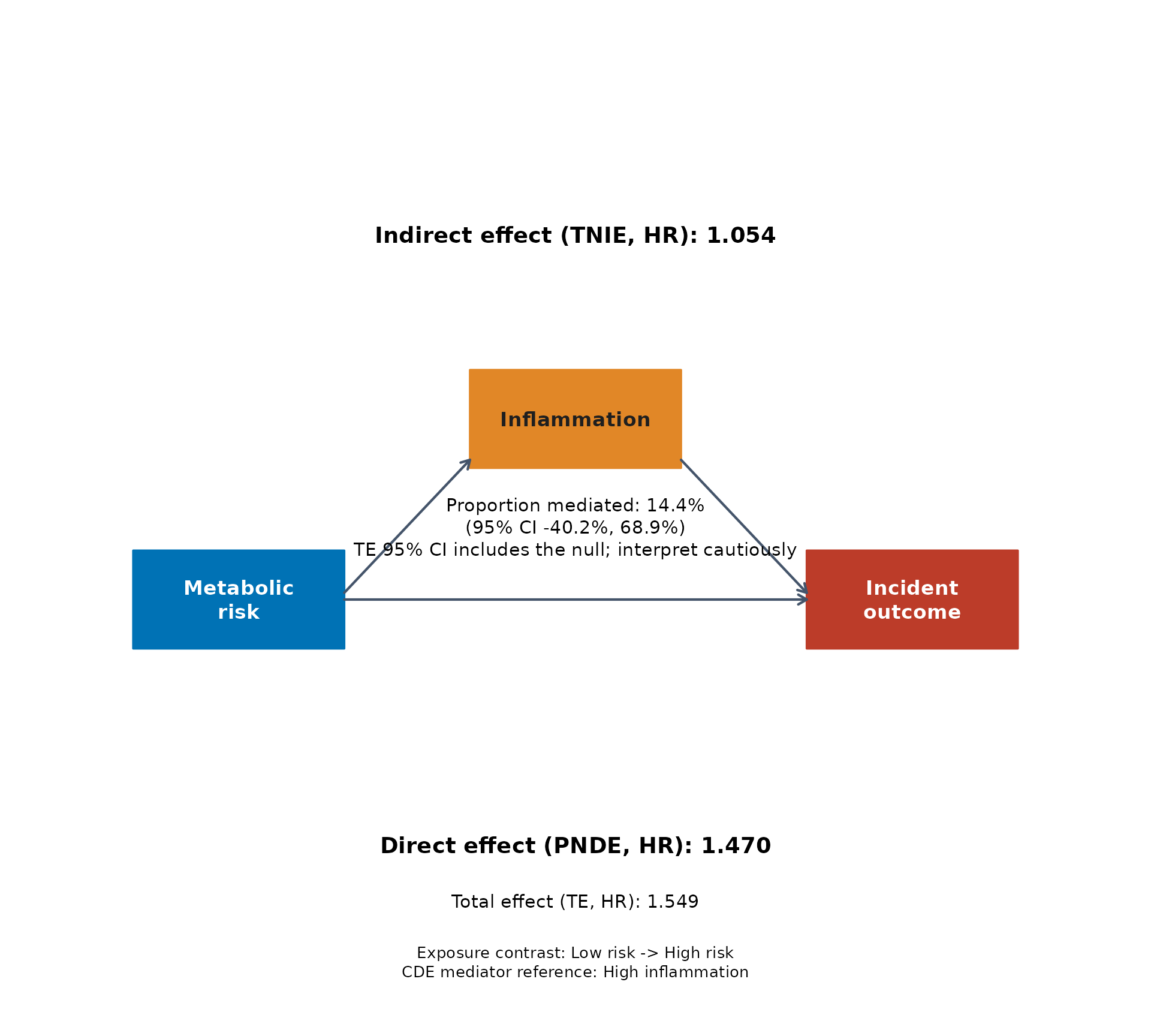
#> 3                  Proportion mediated 14.4% (-40.2% to 68.9%)

Because the event rate in this example is only 6.0%, yreg = "auto" selected survCox, so the ratio scale is a hazard ratio.

In manuscript-style language, the Model B result can be read as:

the High risk group has an overall hazard ratio that is about 54.9% higher than the Low risk group (te = 1.549)
the inflammation pathway contributes only a modest indirect effect (tnie = 1.054)
the point estimate for the proportion mediated is 14.4%, suggesting that part of the overall association could be operating through the inflammation pathway

The critical scientific qualifier is uncertainty. Here the confidence interval for pm is wide and crosses zero, so the careful interpretation is not “mediation has been established”, but:

the estimates are compatible with partial mediation through inflammation, but the pathway effect remains too imprecise to support a strong mechanistic claim on its own

Inspect the evaluation settings directly

leo_cox_mediation() keeps a compact evaluation summary in $evaluation.

res_med$evaluation
#>     model exposure mediator outcome   n case_n non_event_n followup_total
#> 1 Model A exposure mediator outcome 500     30         470       5470.759
#> 2 Model B exposure mediator outcome 500     30         470       5470.759
#>   event_rate     exposure_contrast exposure_contrast_value x_exp_a0 x_exp_a1
#> 1       0.06 Low risk -> High risk          0.000 -> 1.000        0        1
#> 2       0.06 Low risk -> High risk          0.000 -> 1.000        0        1
#>   mediator_reference         x_med_cde x_med_cde_internal     mreg    yreg
#> 1  High inflammation High inflammation                  1 logistic survCox
#> 2  High inflammation High inflammation                  1 logistic survCox
#>   pm_unstable
#> 1        TRUE
#> 2        TRUE
#>                                                                                                                       pm_note
#> 1 Total effect 95% CI includes the null value; proportion mediated (pm) may be unstable and should be interpreted cautiously.
#> 2 Total effect 95% CI includes the null value; proportion mediated (pm) may be unstable and should be interpreted cautiously.
#>   interaction covariates             x_cov_cond
#> 1        TRUE        age             age=59.523
#> 2        TRUE   age, bmi age=59.523; bmi=25.464

This table is especially useful when you want to audit:

which x_exp_a0 -> x_exp_a1 contrast was used
which mediator reference was used for the controlled direct effect
which covariate profile was used for x_cov_cond
which mreg and yreg were used
whether the outcome model included x_exp:x_med

Non-numeric covariates need explicit `x_cov_cond`

When the selected adjustment set contains a non-numeric covariate, the evaluation profile must be given explicitly. The same applies to binary numeric covariates such as 0/1 indicators, because the default median can otherwise create impossible values such as 0.5.

res_med_smoking <- leo_cox_mediation(
  df = med_df,
  y_out = c("outcome", "outcome_censor"),
  x_exp = "exposure",
  x_med = "mediator",
  x_cov = "smoking",
  x_cov_cond = list(smoking = "Never"),
  verbose = FALSE
)

res_med_smoking$evaluation
#>     model exposure mediator outcome   n case_n non_event_n followup_total
#> 1 model_1 exposure mediator outcome 500     30         470       5470.759
#>   event_rate     exposure_contrast exposure_contrast_value x_exp_a0 x_exp_a1
#> 1       0.06 Low risk -> High risk          0.000 -> 1.000        0        1
#>   mediator_reference         x_med_cde x_med_cde_internal     mreg    yreg
#> 1  High inflammation High inflammation                  1 logistic survCox
#>   pm_unstable
#> 1        TRUE
#>                                                                                                                       pm_note
#> 1 Total effect 95% CI includes the null value; proportion mediated (pm) may be unstable and should be interpreted cautiously.
#>   interaction covariates    x_cov_cond
#> 1        TRUE    smoking smoking=Never

This is not just more transparent. It is required whenever x_cov contains a factor or binary numeric covariate, because the evaluation profile has to map to a real person that the reader can reconstruct.

Continuous mediators, including score-like mediators, are also supported

The same workflow can also be used with a continuous mediator.

med_df_cont <- dplyr::mutate(
  med_df,
  mediator_cont = rnorm(
    n,
    mean = 0.5 * as.integer(exposure == "High risk") + 0.02 * (age - 60),
    sd = 1
  )
)

res_med_cont <- leo_cox_mediation(
  df = med_df_cont,
  y_out = c("outcome", "outcome_censor"),
  x_exp = "exposure",
  x_med = "mediator_cont",
  x_cov = "age",
  mreg = "linear",
  verbose = FALSE
)

res_med_cont$result
#>     Model Effect code                        Effect        Scale Exposure
#> 1 model_1         cde      Controlled direct effect Hazard ratio exposure
#> 2 model_1        pnde    Pure natural direct effect Hazard ratio exposure
#> 3 model_1        tnie Total natural indirect effect Hazard ratio exposure
#> 4 model_1        tnde   Total natural direct effect Hazard ratio exposure
#> 5 model_1        pnie  Pure natural indirect effect Hazard ratio exposure
#> 6 model_1          te                  Total effect Hazard ratio exposure
#> 7 model_1          pm           Proportion mediated   Proportion exposure
#>        Mediator Outcome     Exposure contrast Mediator reference   N Case N
#> 1 mediator_cont outcome Low risk -> High risk              0.233 500     30
#> 2 mediator_cont outcome Low risk -> High risk               <NA> 500     30
#> 3 mediator_cont outcome Low risk -> High risk               <NA> 500     30
#> 4 mediator_cont outcome Low risk -> High risk               <NA> 500     30
#> 5 mediator_cont outcome Low risk -> High risk               <NA> 500     30
#> 6 mediator_cont outcome Low risk -> High risk               <NA> 500     30
#> 7 mediator_cont outcome Low risk -> High risk               <NA> 500     30
#>   Non-event N Total follow-up Estimate        95% CI P value Mediator model
#> 1         470        5470.759    1.562  0.760, 3.213   0.225         linear
#> 2         470        5470.759    1.694  0.801, 3.584   0.168         linear
#> 3         470        5470.759    0.917  0.775, 1.086   0.315         linear
#> 4         470        5470.759    1.554  0.747, 3.233   0.238         linear
#> 5         470        5470.759    1.000  0.849, 1.178   0.999         linear
#> 6         470        5470.759    1.554  0.755, 3.201   0.231         linear
#> 7         470        5470.759   -0.252 -0.849, 0.345   0.407         linear
#>   Outcome model
#> 1       survCox
#> 2       survCox
#> 3       survCox
#> 4       survCox
#> 5       survCox
#> 6       survCox
#> 7       survCox

For a continuous mediator, the cde row shows a numeric mediator reference because the controlled direct effect is evaluated at x_med_cde.

This is also the workflow we would usually recommend for an ordered score-like mediator. For example, if a low-grade inflammation index ranges from -7 to 7, the first question is scientific rather than computational:

does the index behave like a severity score, where one-unit changes are interpretable enough for a linear approximation?
or is the real question about a thresholded state that should be defined as binary first?

For most ordered severity scores, the cleaner first pass is to keep the score numeric and fit a linear mediator model.

Add a paper-style pathway figure

For a single mediator, a compact pathway figure often communicates the result faster than a dense table alone.

leo_cox_mediation_plot(
  x = res_med,
  model = "Model B",
  exposure_label = "Metabolic\nrisk",
  mediator_label = "Inflammation",
  outcome_label = "Incident\noutcome",
  language = "en",
  palette = "jama"
)

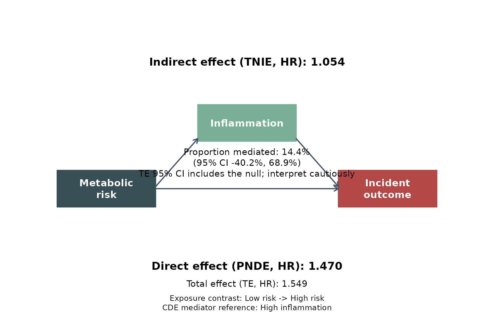
This figure is useful because it keeps the main teaching elements in one place:

left box: the exposure contrast
middle box: the proposed mediator
right box: the incident outcome
top text: the indirect pathway through the mediator
middle text: the estimated proportion of the total effect attributed to that pathway
bottom text: the direct pathway not explained by the mediator

One subtle but important point is that the mediated pathway shown here is the full X -> M -> Y pathway. The figure does not print a separate M -> Y coefficient because regmedint reports causal decomposition quantities such as tnie, pnde, and te, rather than a simple product of two regression coefficients.

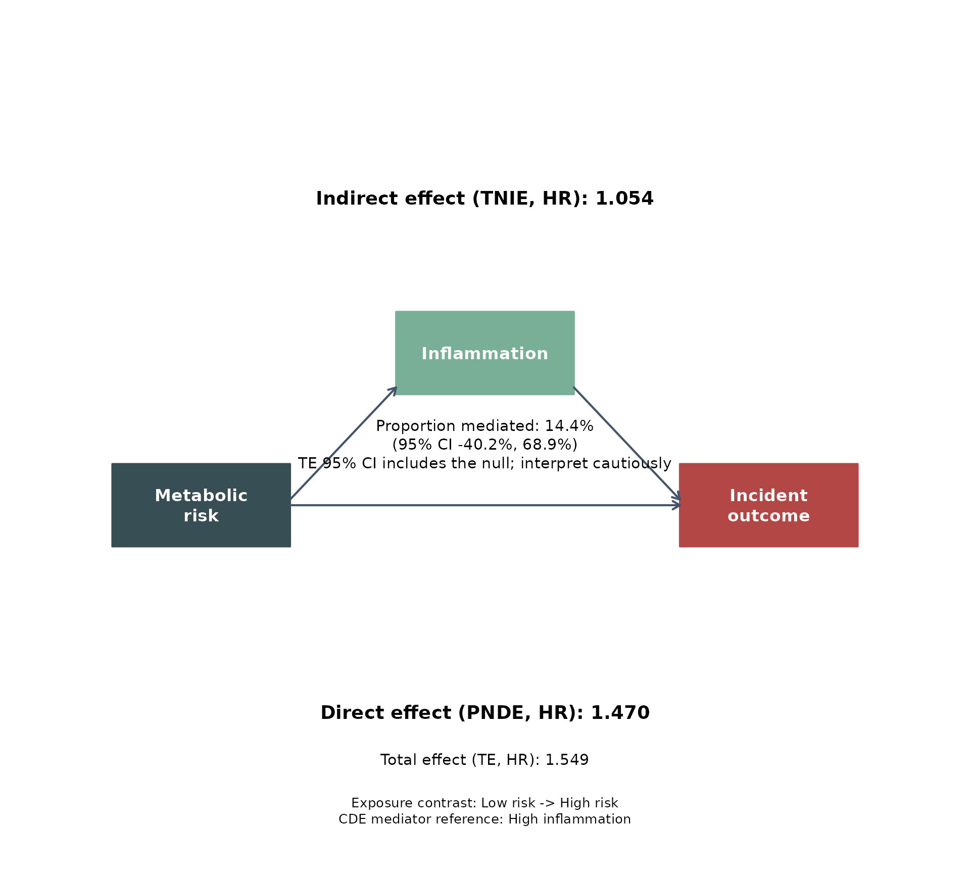
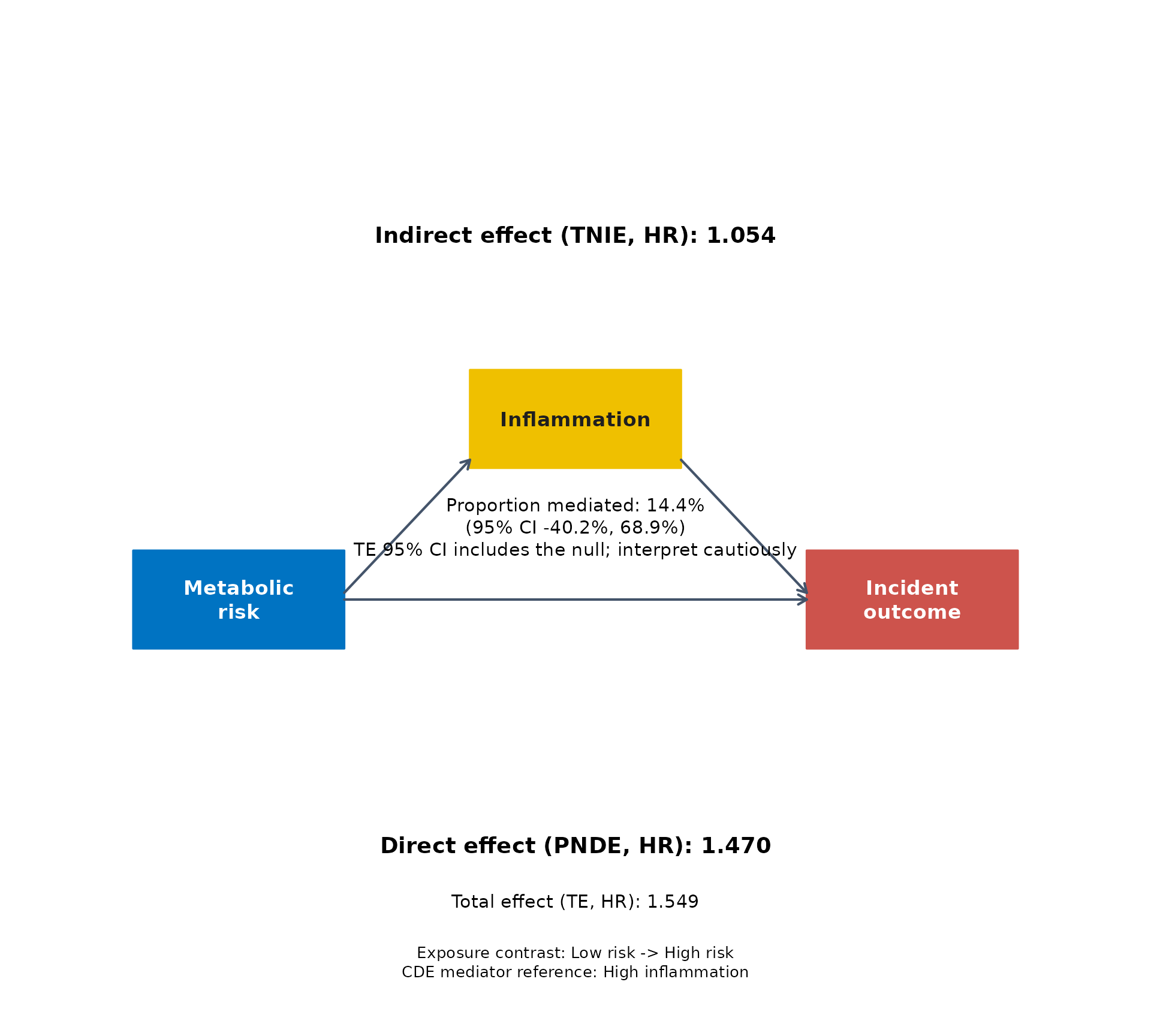
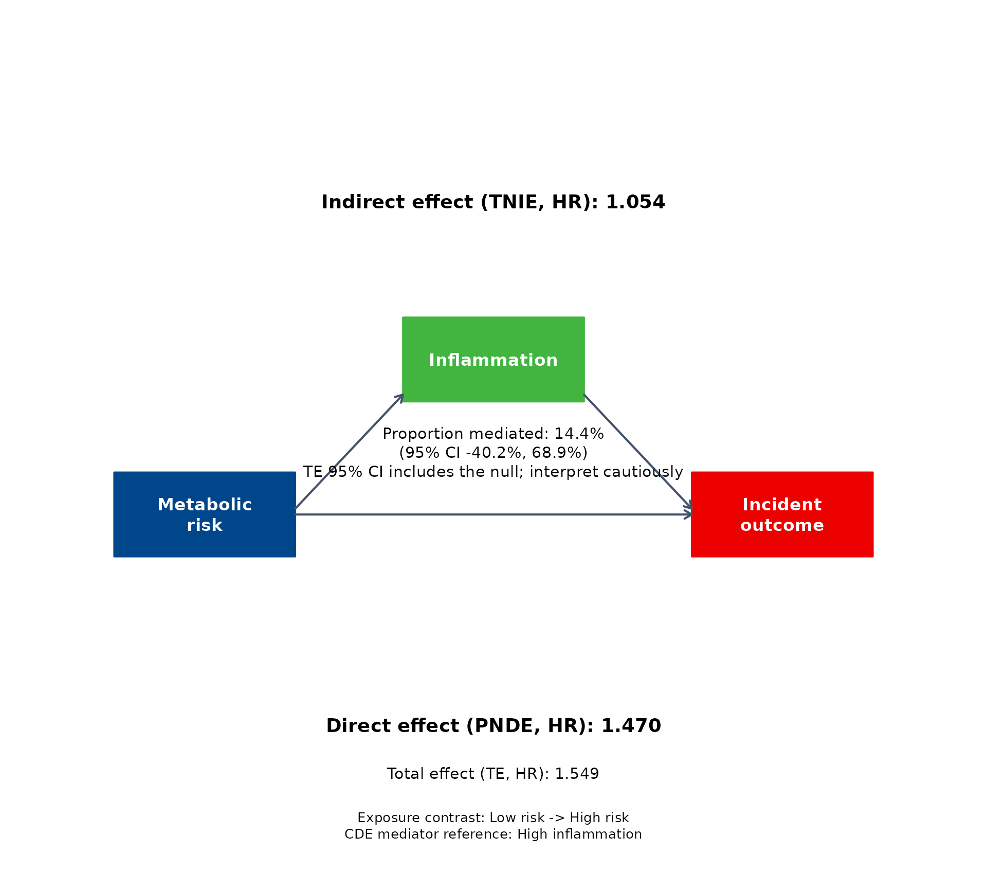
Compare the built-in journal palettes

The same fitted result can be displayed with several built-in journal-style palettes.

for (pal in c("jama", "jco", "lancet", "nejm")) {
  leo_cox_mediation_plot(
    x = res_med,
    model = "Model B",
    exposure_label = "Metabolic\nrisk",
    mediator_label = "Inflammation",
    outcome_label = "Incident\noutcome",
    language = "en",
    palette = pal
  )
}

How to interpret common result patterns

In applied survival mediation analysis, the most common interpretation patterns are:

te is clearly away from the null, tnie is modest, and pm is positive but imprecise: compatible with partial mediation, but not decisive
te and tnie are both clearly away from the null, and pm is precise: stronger evidence that the pathway may explain a meaningful share of the total effect
te is weak or crosses the null: pm can become unstable and should be treated cautiously
yreg switches to AFT: all non-pm effect rows should now be interpreted as time ratios rather than hazard ratios

This is why Step 3 is not only about producing a decomposition table. It is also about learning when the estimates are scientifically interpretable and when they are still too unstable for a strong claim.

How to write this in a paper

A defensible reporting order is usually:

report the main exposure-outcome association first
then present the mediation analysis as a pathway decomposition
state the exposure contrast, mediator reference, and adjustment profile
report which yreg was used; if it was survCox, mention the rare-event approximation and make clear that this means the decomposition is only being reported as an approximate split when events are relatively rare, and if it was AFT, remember that the ratio scale is a time ratio
if exposure and mediator are measured at the same baseline visit, write the result up as decomposition evidence that is consistent with an assumed pathway, and say explicitly that the data alone do not establish exposure before mediator unless temporal ordering is supported externally

In other words, mediation should usually refine the biological story after the main Cox result is already established.

What to take away from Step 3

This step should leave you with six practical rules:

mediation asks a pathway question, not a heterogeneity question
the data should be checked before fitting, just as in Step 1 and Step 2
x_exp_a0, x_exp_a1, x_med_cde, and x_cov_cond define where the mediation effects are evaluated
mreg controls x_med ~ x_exp + x_cov, yreg controls time ~ x_exp + x_med + x_cov, and interaction = TRUE adds x_exp:x_med to the outcome model
yreg = "auto" chooses survCox for event proportion <= 10% (which means the decomposition then relies on the rare-event approximation and is better read as approximate when events are relatively rare) and survAFT_weibull otherwise
factor mediators should not be forced into mreg = "linear", and the final mediation result should always be interpreted with the actual outcome model, uncertainty, and the study’s temporal ordering in mind