Survival Analysis Step 3.1: Mediation Case Study

Why this article exists

Step 3.0 explains what mediation analysis is for. Step 3.1 is where we turn that into a practical workflow.

The goal here is not just to run leo_cox_mediation(), but to answer five questions in a way that stays tied to real output:

1. what biological question are we actually asking?
2. how do x_exp_a0, x_exp_a1, x_med_cde, and x_cov_cond map to that question?
3. when should mreg = "linear" be preferred over mreg = "logistic"?
4. what changes when yreg = "auto" switches from survCox to survAFT_weibull?
5. how should the scientific interpretation change across those settings?

Build one reproducible scientific story, then vary the scenario

We use a synthetic cohort with the same broad question throughout:

is the association between higher metabolic risk and an incident outcome partly explained by inflammation?

The scenarios differ only in how we encode the mediator and how common the outcome is.

set.seed(20260324)

make_mediation_case <- function(n = 1500, base_log_hazard = -5.8, censor_rate = 0.06) {
  age <- rnorm(n, 60, 8)
  sex <- factor(sample(c("Female", "Male"), n, replace = TRUE))
  smoking <- factor(sample(c("Never", "Ever"), n, replace = TRUE, prob = c(0.6, 0.4)))
  sex_num <- as.integer(sex == "Male")
  smoking_num <- as.integer(smoking == "Ever")
  metabolic_risk_num <- rbinom(
    n, 1,
    plogis(-0.3 + 0.03 * (age - 60) + 0.30 * sex_num + 0.35 * smoking_num)
  )
  inflammation_score <- rnorm(
    n,
    mean = 0.85 * metabolic_risk_num + 0.04 * (age - 60) + 0.35 * smoking_num,
    sd = 0.9
  )
  hazard_rate <- exp(
    base_log_hazard +
      0.55 * metabolic_risk_num +
      0.24 * inflammation_score +
      0.02 * (age - 60) +
      0.20 * smoking_num
  )
  event_time <- rexp(n, rate = hazard_rate)
  censor_time <- rexp(n, rate = censor_rate)

  data.frame(
    incident_event = as.integer(event_time <= censor_time),
    followup_years = pmin(event_time, censor_time),
    metabolic_risk = factor(
      metabolic_risk_num,
      levels = c(0, 1),
      labels = c("Lower risk", "Higher risk")
    ),
    inflammation_score = inflammation_score,
    inflammation_group = factor(
      as.integer(inflammation_score > 0.5),
      levels = c(0, 1),
      labels = c("Lower inflammation", "Higher inflammation")
    ),
    age = age,
    sex = sex,
    smoking = smoking
  )
}

rare_case <- make_mediation_case(base_log_hazard = -5.8, censor_rate = 0.06)
common_case <- make_mediation_case(base_log_hazard = -4.6, censor_rate = 0.06)

data.frame(
  Scenario = c("Rare-outcome case", "Common-outcome case"),
  Participants = c(nrow(rare_case), nrow(common_case)),
  Events = c(sum(rare_case$incident_event), sum(common_case$incident_event)),
  `Event rate` = c(fmt_pct(mean(rare_case$incident_event)), fmt_pct(mean(common_case$incident_event)))
)
#>              Scenario Participants Events Event.rate
#> 1   Rare-outcome case         1500    131       8.7%
#> 2 Common-outcome case         1500    339      22.6%

The rare-outcome case will let yreg = "auto" stay on survCox, because the post-filter, complete-case analysis set still has an event rate at or below 10%. The common-outcome case is deliberately built to push the same scientific question onto the AFT path.

Case 1. A graded biomarker mediator in a rare-outcome setting

This is the most natural scenario when inflammation is scientifically treated as a continuum rather than as a yes/no threshold.

x_med_cde_case1 <- stats::median(rare_case$inflammation_score, na.rm = TRUE)

res_case1 <- leo_cox_mediation(
  df = rare_case,
  y_out = c("incident_event", "followup_years"),
  x_exp = "metabolic_risk",
  x_med = "inflammation_score",
  x_cov = c("age", "sex", "smoking"),
  x_exp_a0 = 0,
  x_exp_a1 = 1,
  x_med_cde = x_med_cde_case1,
  x_cov_cond = list(age = 60, sex = "Female", smoking = "Never"),
  mreg = "linear",
  yreg = "auto",
  interaction = TRUE,
  verbose = FALSE
)

case1_eval <- res_case1$evaluation
case1_te <- get_effect_row(res_case1, "te")
case1_tnie <- get_effect_row(res_case1, "tnie")
case1_pm <- get_effect_row(res_case1, "pm")
case1_te_ci <- case1_te[["95% CI"]][1]
case1_tnie_ci <- case1_tnie[["95% CI"]][1]
case1_pm_ci <- case1_pm[["95% CI"]][1]

Read the evaluation settings before reading the effects

res_case1$evaluation[, c(
  "exposure_contrast", "x_exp_a0", "x_exp_a1",
  "mediator_reference", "x_med_cde", "x_cov_cond",
  "mreg", "yreg", "interaction"
)]
#>           exposure_contrast x_exp_a0 x_exp_a1 mediator_reference x_med_cde
#> 1 Lower risk -> Higher risk        0        1              0.568 0.5680312
#>                              x_cov_cond   mreg    yreg interaction
#> 1 age=60.000; sex=Female; smoking=Never linear survCox        TRUE

This one table already answers the three user-facing evaluation questions:

• x_exp_a0 = 0, x_exp_a1 = 1 means we are comparing Lower risk -> Higher risk
• x_med_cde = 0.568 means the controlled direct effect is being evaluated at the median inflammation score
• x_cov_cond = age=60; sex=Female; smoking=Never means the reported effects are evaluated for that covariate profile, not as a profile-free population average

In plain language, the CDE here asks:

if two otherwise similar 60-year-old never-smoking women differed only in metabolic-risk status, but both were fixed at an inflammation score of 0.568, how different would their outcome risk be?

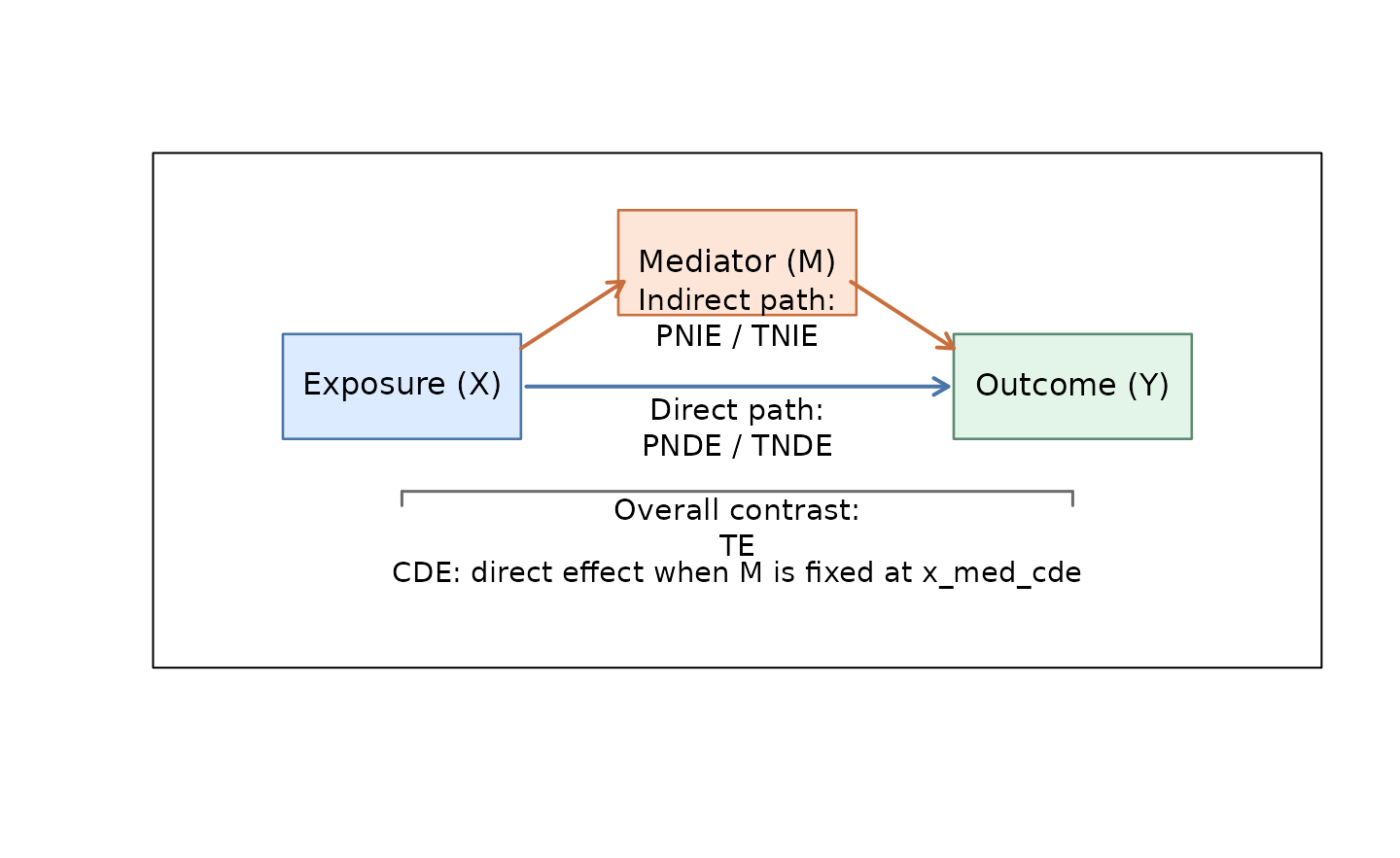
Keep one simple map of the effect names in mind

Code	Full name	How to read it
TE	Total Effect	the overall association
TNIE	Total Natural Indirect Effect	the part that travels through the mediator
PNDE	Pure Natural Direct Effect	the part that does not travel through the mediator
PM	Proportion Mediated	the share of the total effect attributed to the mediator pathway
CDE	Controlled Direct Effect	the direct effect when the mediator is fixed at x_med_cde
TNDE	Total Natural Direct Effect	an alternative natural direct-effect definition
PNIE	Pure Natural Indirect Effect	an alternative natural indirect-effect definition

For most papers, the first pass is usually TE, TNIE, PNDE, and PM. CDE becomes important when the scientific question is explicitly about fixing the mediator at a chosen level.

That is also why Mediator reference appears only in the cde row: only the controlled direct effect needs a fixed mediator value.

Visualize the biology before over-interpreting the decomposition

First look at whether the mediator really behaves like a graded biomarker across the two exposure groups.

ggplot2::ggplot(
  rare_case,
  ggplot2::aes(x = metabolic_risk, y = inflammation_score, fill = metabolic_risk)
) +
  ggplot2::geom_violin(trim = FALSE, alpha = 0.35, color = NA) +
  ggplot2::geom_boxplot(width = 0.16, outlier.alpha = 0.15, color = "#1f1f1f") +
  ggplot2::scale_fill_manual(values = c("#5B8FF9", "#D14A61")) +
  ggplot2::labs(
    title = "Inflammation score is shifted upward in the higher-risk group",
    x = "Metabolic risk group",
    y = "Inflammation score"
  ) +
  ggplot2::theme_minimal(base_size = 12) +
  ggplot2::theme(legend.position = "none")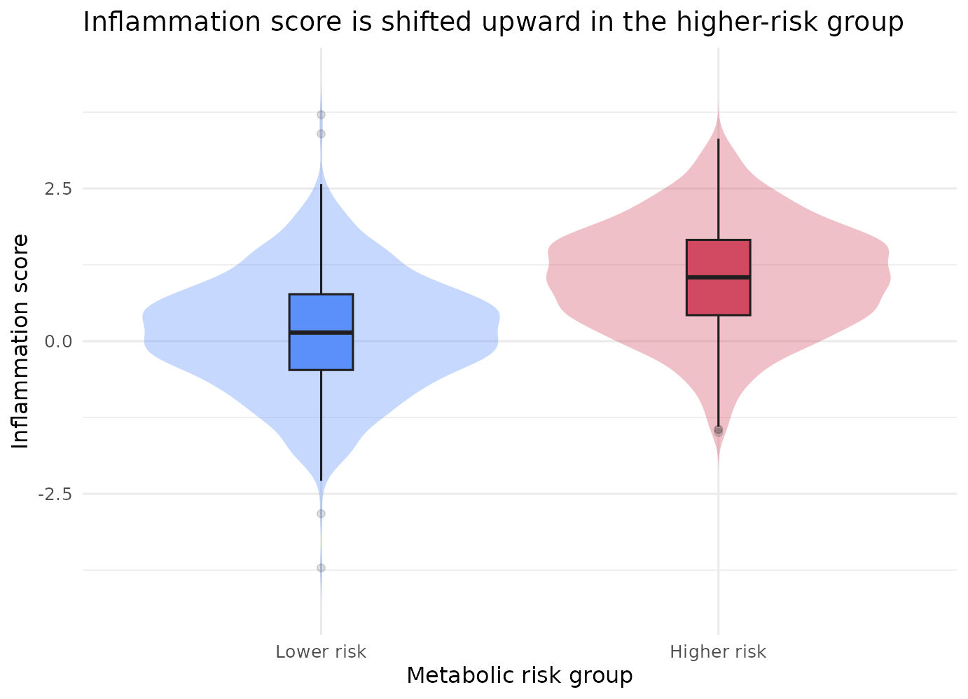

Now look at the crude joint pattern that motivates keeping interaction = TRUE in the outcome model.

joint_event_case1 <- dplyr::summarise(
  dplyr::group_by(rare_case, metabolic_risk, inflammation_group),
  n = dplyr::n(),
  event_rate = mean(incident_event),
  .groups = "drop"
)

ggplot2::ggplot(
  joint_event_case1,
  ggplot2::aes(x = inflammation_group, y = event_rate, fill = metabolic_risk)
) +
  ggplot2::geom_col(position = ggplot2::position_dodge(width = 0.7), width = 0.62) +
  ggplot2::geom_text(
    ggplot2::aes(label = paste0(fmt_pct(event_rate), "\n(n=", n, ")")),
    position = ggplot2::position_dodge(width = 0.7),
    vjust = -0.15,
    size = 3.3
  ) +
  ggplot2::scale_fill_manual(values = c("#5B8FF9", "#D14A61")) +
  ggplot2::scale_y_continuous(
    labels = function(x) paste0(round(100 * x), "%"),
    limits = c(0, max(joint_event_case1$event_rate) * 1.18)
  ) +
  ggplot2::labs(
    title = "The highest crude event rate appears in the higher-risk plus higher-inflammation stratum",
    x = "Inflammation group",
    y = "Observed event rate",
    fill = "Metabolic risk"
  ) +
  ggplot2::theme_minimal(base_size = 12)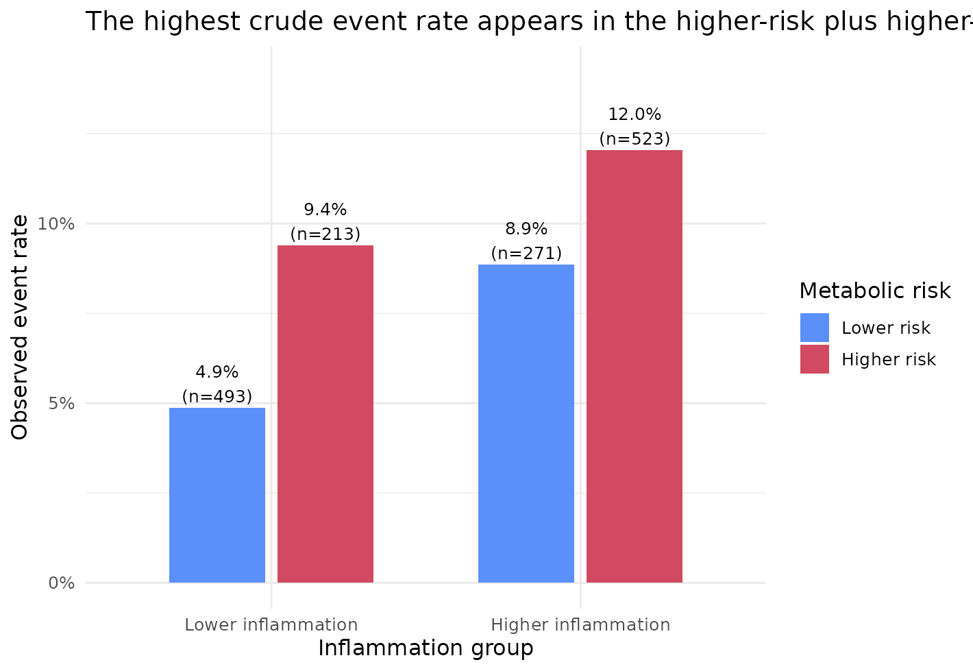

That figure does not prove interaction by itself, but it shows why the default interaction = TRUE is often a sensible first pass: it avoids forcing the effect of metabolic risk to be identical at every inflammation level.

Interpret the actual mediation result, not an imagined one

dplyr::filter(res_case1$result, `Effect code` %in% c("te", "tnie", "pm"))
#>     Model Effect code                        Effect        Scale       Exposure
#> 1 model_1        tnie Total natural indirect effect Hazard ratio metabolic_risk
#> 2 model_1          te                  Total effect Hazard ratio metabolic_risk
#> 3 model_1          pm           Proportion mediated   Proportion metabolic_risk
#>             Mediator        Outcome         Exposure contrast
#> 1 inflammation_score incident_event Lower risk -> Higher risk
#> 2 inflammation_score incident_event Lower risk -> Higher risk
#> 3 inflammation_score incident_event Lower risk -> Higher risk
#>   Mediator reference    N Case N Non-event N Total follow-up Estimate
#> 1               <NA> 1500    131        1369        23086.95    1.246
#> 2               <NA> 1500    131        1369        23086.95    1.877
#> 3               <NA> 1500    131        1369        23086.95    0.423
#>         95% CI P value Mediator model Outcome model
#> 1 1.018, 1.525   0.033         linear       survCox
#> 2 1.303, 2.703  <0.001         linear       survCox
#> 3 0.027, 0.820   0.036         linear       survCox

Because this rare-outcome scenario stayed on survCox, the ratio scale is a hazard ratio.

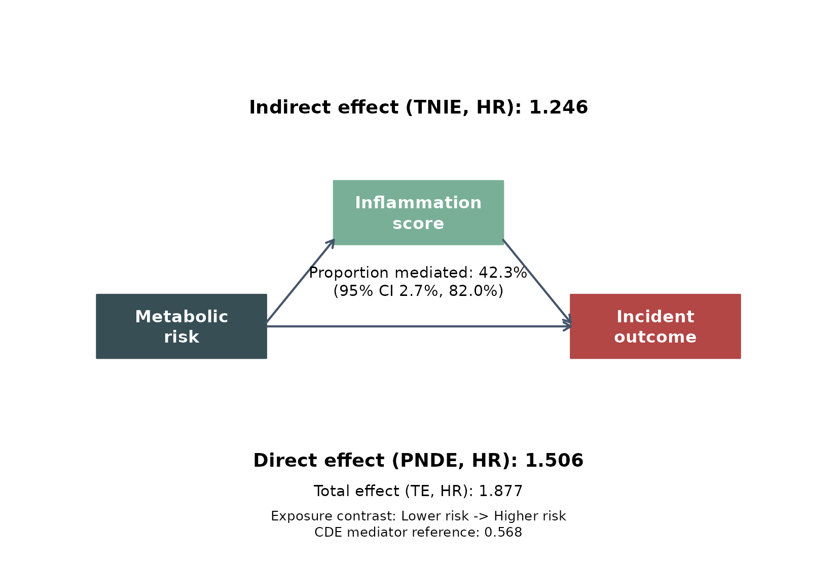
In this fitted example:

• the total effect was 1.877 (1.303, 2.703), meaning the higher-risk group had a substantially higher incident hazard overall
• the indirect pathway through the continuous inflammation score was 1.246 (1.018, 1.525), so the mediator pathway itself still points in the same harmful direction
• the estimated proportion mediated was 42.3% (0.027, 0.820), suggesting that inflammation may explain a sizeable share of the total association in this synthetic cohort

Here the pm confidence interval stays above 0, so this particular simulated example is more consistent with a positive mediated share than with a null mediated contribution.

Scientifically, that is the pattern we would describe as:

higher metabolic risk is associated with both a higher inflammation burden and a higher incident hazard, and the mediation decomposition is compatible with inflammation carrying a meaningful part of that pathway.

The pathway figure makes the same result easier to communicate in a paper or slide deck.

leo_cox_mediation_plot(
  x = res_case1,
  exposure_label = "Metabolic\nrisk",
  mediator_label = "Inflammation\nscore",
  outcome_label = "Incident\noutcome",
  language = "en",
  palette = "jama"
)

Case 2. The same biology, but a thresholded binary mediator

Sometimes the scientific question is about a thresholded inflammatory state rather than a graded biomarker. The model then changes from mreg = "linear" to mreg = "logistic".

res_case2 <- leo_cox_mediation(
  df = rare_case,
  y_out = c("incident_event", "followup_years"),
  x_exp = "metabolic_risk",
  x_med = "inflammation_group",
  x_cov = c("age", "sex", "smoking"),
  x_exp_a0 = 0,
  x_exp_a1 = 1,
  x_med_cde = "Higher inflammation",
  x_cov_cond = list(age = 60, sex = "Female", smoking = "Never"),
  mreg = "logistic",
  yreg = "auto",
  interaction = TRUE,
  verbose = FALSE
)

case2_tnie <- get_effect_row(res_case2, "tnie")
case2_pm <- get_effect_row(res_case2, "pm")

dplyr::bind_rows(
  case_summary_row(res_case1, "Case 1: rare outcome + continuous mediator"),
  case_summary_row(res_case2, "Case 2: rare outcome + binary mediator")
)
#>                                     Scenario Event rate Outcome model
#> 1 Case 1: rare outcome + continuous mediator       8.7%       survCox
#> 2     Case 2: rare outcome + binary mediator       8.7%       survCox
#>           Total effect      Indirect effect   Proportion mediated
#> 1 1.877 (1.303, 2.703) 1.246 (1.018, 1.525)   42.3% (2.7%, 82.0%)
#> 2 1.878 (1.304, 2.706) 1.100 (0.920, 1.315) 19.5% (-16.4%, 55.4%)

The scientific lesson is not that binary mediators are wrong. It is that the mediator encoding should match the question. For logistic mediators, x_med_cde should now be given as the original observed mediator level, not an internal 0/1 recode:

• in Case 1, the indirect pathway was 1.246 on the hazard-ratio scale, with pm estimated at 42.3%
• in Case 2, the same broad story became much weaker and less precise (tnie = 1.100, pm = 19.5%)

That is a useful teaching contrast. If the biology is genuinely graded, turning the mediator into a yes/no label can discard pathway information. If the real question is threshold-based, however, the binary mediator may be the better scientific choice even if it is statistically less efficient.

Case 3. The same pathway question, but with a more common outcome

Now keep the same exposure-mediator story and only make the event more common. This is where yreg = "auto" becomes important.

res_case3 <- leo_cox_mediation(
  df = common_case,
  y_out = c("incident_event", "followup_years"),
  x_exp = "metabolic_risk",
  x_med = "inflammation_score",
  x_cov = c("age", "sex", "smoking"),
  x_exp_a0 = 0,
  x_exp_a1 = 1,
  x_med_cde = stats::median(common_case$inflammation_score, na.rm = TRUE),
  x_cov_cond = list(age = 60, sex = "Female", smoking = "Never"),
  mreg = "linear",
  yreg = "auto",
  interaction = TRUE,
  verbose = FALSE
)

case3_te <- get_effect_row(res_case3, "te")
case3_tnie <- get_effect_row(res_case3, "tnie")
case3_pm <- get_effect_row(res_case3, "pm")

res_case3$evaluation[, c("event_rate", "mreg", "yreg", "interaction", "x_cov_cond")]
#>   event_rate   mreg            yreg interaction
#> 1      0.226 linear survAFT_weibull        TRUE
#>                              x_cov_cond
#> 1 age=60.000; sex=Female; smoking=Never
dplyr::filter(res_case3$result, `Effect code` %in% c("te", "tnie", "pm"))
#>     Model Effect code                        Effect      Scale       Exposure
#> 1 model_1        tnie Total natural indirect effect Time ratio metabolic_risk
#> 2 model_1          te                  Total effect Time ratio metabolic_risk
#> 3 model_1          pm           Proportion mediated Proportion metabolic_risk
#>             Mediator        Outcome         Exposure contrast
#> 1 inflammation_score incident_event Lower risk -> Higher risk
#> 2 inflammation_score incident_event Lower risk -> Higher risk
#> 3 inflammation_score incident_event Lower risk -> Higher risk
#>   Mediator reference    N Case N Non-event N Total follow-up Estimate
#> 1               <NA> 1500    339        1161         19723.5    0.860
#> 2               <NA> 1500    339        1161         19723.5    0.396
#> 3               <NA> 1500    339        1161         19723.5    0.107
#>          95% CI P value Mediator model   Outcome model
#> 1  0.754, 0.981   0.024         linear survAFT_weibull
#> 2  0.303, 0.518  <0.001         linear survAFT_weibull
#> 3 -0.011, 0.225   0.076         linear survAFT_weibull

Here the event rate was 22.6%, so yreg = "auto" switched to survAFT_weibull.

That changes the interpretation scale:

• te = 0.396 is now a time ratio, not a hazard ratio
• because the time ratio is below 1, the higher-risk group has shorter event-free time
• tnie = 0.860 means the inflammation pathway is also pointing toward shorter event-free time

This is the same biological story on a different model scale. The key practical point is that the wording must change with yreg:

• survCox: talk about higher or lower hazard
• survAFT_weibull: talk about shorter or longer event-free time

Put the three scenarios side by side

dplyr::bind_rows(
  case_summary_row(res_case1, "Case 1: rare outcome + continuous mediator"),
  case_summary_row(res_case2, "Case 2: rare outcome + binary mediator"),
  case_summary_row(res_case3, "Case 3: common outcome + continuous mediator")
)
#>                                       Scenario Event rate   Outcome model
#> 1   Case 1: rare outcome + continuous mediator       8.7%         survCox
#> 2       Case 2: rare outcome + binary mediator       8.7%         survCox
#> 3 Case 3: common outcome + continuous mediator      22.6% survAFT_weibull
#>           Total effect      Indirect effect   Proportion mediated
#> 1 1.877 (1.303, 2.703) 1.246 (1.018, 1.525)   42.3% (2.7%, 82.0%)
#> 2 1.878 (1.304, 2.706) 1.100 (0.920, 1.315) 19.5% (-16.4%, 55.4%)
#> 3 0.396 (0.303, 0.518) 0.860 (0.754, 0.981)  10.7% (-1.1%, 22.5%)

This comparison is useful because it separates three different decisions:

1. how to define the mediator scientifically
2. how much information is lost when a graded mediator is dichotomized
3. how the interpretation scale changes when the outcome is no longer rare

Key practical takeaways

If you only keep six practical rules from Step 3.1, make them these:

1. choose x_exp_a0 and x_exp_a1 to match the exposure contrast you would actually write in a Results section
2. choose x_med_cde to represent the mediator level at which you want the controlled direct effect to be interpreted; for continuous biomarkers, the median is often a clean first choice
3. choose x_cov_cond to represent a real covariate profile, especially when x_cov includes factor variables
4. use mreg = "linear" when the mediator is scientifically graded, and mreg = "logistic" when the mediator question is genuinely threshold-based
5. let yreg = "auto" protect you from using survCox in obviously non-rare settings, but always read the final Outcome model before interpreting the ratio scale
6. write the scientific conclusion from the actual fitted output, not from the existence of a pathway diagram or a single positive point estimate