生存分析 Step 3.0:中介分析
survival-analysis-step3-zh.Rmd这一步要解决什么问题
这篇教程是 leo.ukb 生存分析部分的 Step 3.0。完成主 Cox
分析,以及 Step 2 里的亚组/交互分析之后,下一类常见问题是:
exposure 和结局之间的关联,有没有一部分是通过某个 mediator 传递的?
这就是中介分析,不是亚组分析,也不是交互分析。
先把中介分析和交互分析分清楚
当前这套生存分析 workflow 其实是在回答三类不同的问题:
- Step 1:有没有主 exposure-outcome 关联?
- Step 2:这个关联会不会在不同人群里不一样,又该在哪个尺度上解释?
- Step 3.0:这个关联是不是部分通过 mediator 路径传递?
所以:
- interaction 讨论的是 效应异质性
- mediation 讨论的是 路径分解
中介分析不是替代 Step 1/Step 2,而是在前两步成立以后进一步细化生物学故事。
先从数据和变量角色开始
下面继续用一个教学型模拟数据:rare event、二分类 exposure、二分类 mediator, 再加几个常见协变量。
set.seed(20260323)
n <- 500
age <- rnorm(n, 60, 8)
bmi <- rnorm(n, 26, 4)
smoking <- factor(sample(c("Never", "Ever"), n, replace = TRUE))
exposure_num <- rbinom(n, 1, plogis(-0.2 + 0.02 * (age - 60)))
mediator_num <- rbinom(n, 1, plogis(-0.5 + 0.9 * exposure_num + 0.02 * (bmi - 26)))
hazard_rate <- exp(
  -5.8 + 0.55 * exposure_num + 0.40 * mediator_num +
    0.02 * (age - 60) + 0.03 * (bmi - 26) + 0.20 * (smoking == "Ever")
)
event_time <- rexp(n, rate = hazard_rate)
censor_time <- rexp(n, rate = 0.08)

med_df <- data.frame(
  outcome = as.integer(event_time <= censor_time),
  outcome_censor = pmax(pmin(event_time, censor_time), 0.2),
  exposure = factor(exposure_num, levels = c(0, 1), labels = c("Low risk", "High risk")),
  mediator = factor(
    mediator_num,
    levels = c(0, 1),
    labels = c("Low inflammation", "High inflammation")
  ),
  age = age,
  bmi = bmi,
  smoking = smoking
)
先明确每列变量在 Step 3 里到底扮演什么角色。
dplyr::glimpse(med_df)
#> Rows: 500
#> Columns: 7
#> $ outcome        <int> 0, 0, 0, 0, 0, 0, 0, 0, 0, 0, 0, 0, 1, 1, 0, 0, 0, 0, 0…
#> $ outcome_censor <dbl> 2.6117515, 6.4186284, 8.6449270, 5.6413310, 12.1900483,…
#> $ exposure       <fct> High risk, High risk, Low risk, High risk, Low risk, Lo…
#> $ mediator       <fct> Low inflammation, High inflammation, Low inflammation, …
#> $ age            <dbl> 59.73588, 59.19772, 45.83227, 57.49797, 46.83760, 55.76…
#> $ bmi            <dbl> 27.17832, 27.91178, 30.48299, 24.70933, 22.63096, 28.43…
#> $ smoking <fct> Never, Never, Never, Never, Never, Ever, Ever, Ever, Ev…| 变量 | 类型 | Step 3 角色 |
|---|---|---|
outcome |
二分类事件指示变量 |
incident outcome 是否发生 |
outcome_censor |
随访时间 |
incident outcome 随访时间 |
exposure |
二分类 exposure | 需要被分解的 exposure |
mediator |
二分类 mediator | 候选中介路径变量 |
age |
连续协变量 | 调整协变量 |
bmi |
连续协变量 | 调整协变量 |
smoking |
二分类协变量 | 需要显式指定 x_cov_cond 的示例协变量 |
建模前先看一眼分析数据
和 Step 1、Step 2 一样,真正进入模型之前,先看分析数据是否像样。
| outcome | outcome_censor | exposure | mediator | age | bmi | smoking |
|---|---|---|---|---|---|---|
| 0 | 2.611752 | High risk | Low inflammation | 59.73588 | 27.17832 | Never |
| 0 | 6.418628 | High risk | High inflammation | 59.19772 | 27.91178 | Never |
| 0 | 8.644927 | Low risk | Low inflammation | 45.83227 | 30.48299 | Never |
| 0 | 5.641331 | High risk | Low inflammation | 57.49797 | 24.70933 | Never |
| 0 | 12.190048 | Low risk | Low inflammation | 46.83760 | 22.63096 | Never |
| 0 | 20.568418 | Low risk | Low inflammation | 55.76899 | 28.43722 | Ever |
event_summary <- data.frame(
  指标 = c("Participants", "Events", "Event rate"),
  数值 = c(
    nrow(med_df),
    sum(med_df$outcome),
    sprintf("%.1f%%", 100 * mean(med_df$outcome))
  )
)

knitr::kable(
  event_summary,
  caption = "中介分析教学数据的总体事件负担"
)| 指标 | 数值 |
|---|---|
| Participants | 500 |
| Events | 30 |
| Event rate | 6.0% |
| exposure | mediator | n |
|---|---|---|
| Low risk | Low inflammation | 163 |
| Low risk | High inflammation | 105 |
| High risk | Low inflammation | 102 |
| High risk | High inflammation | 130 |
这几步已经能先回答三个关键问题:
- 事件率是否足够低,以支持
yreg = "auto"走survCox - exposure 和 mediator 的分布是否存在与中介路径一致的模式
- 协变量是否足够可解释,后面能不能定义一个可复现的评价点
建模前先决定中介分析的设置
中介分析最容易被误解的,不是公式,而是“这些效应到底是在什么设定下被评价的”。
setup_table <- data.frame(
  组成部分 = c(
    "Exposure contrast",
    "Mediator 类型",
    "Outcome model",
    "协变量评价点"
  ),
  当前教学规则 = c(
    "优先用二分类 exposure;如果是数值 exposure,就显式给 x_exp_a0 和 x_exp_a1",
    "二分类 mediator -> logistic;连续/评分型 mediator -> linear",
    "yreg = 'auto' 在事件率 <= 10% 时用 survCox,否则用 survAFT_weibull",
    "如果 x_cov 含非数值或二值数值变量,应显式给 x_cov_cond"
  ),
  为什么重要 = c(
    "所有直接/间接效应都围绕这个 exposure 比较定义",
    "Mediator model 决定路径是如何被表示的",
    "最终效应量到底是 HR 还是 TR,取决于 outcome model",
    "中介分解永远是在某个具体协变量人群画像下评价的"
  )
)

knitr::kable(
  setup_table,
  caption = "中介分析建模前的关键设置"
)| 组成部分 | 当前教学规则 | 为什么重要 |
|---|---|---|
| Exposure contrast | 优先用二分类 exposure;如果是数值 exposure,就显式给 x_exp_a0 和 x_exp_a1 | 所有直接/间接效应都围绕这个 exposure 比较定义 |
| Mediator 类型 | 二分类 mediator -> logistic;连续/评分型 mediator -> linear | Mediator model 决定路径是如何被表示的 |
| Outcome model | yreg = ‘auto’ 在事件率 <= 10% 时用 survCox,否则用 survAFT_weibull | 最终效应量到底是 HR 还是 TR,取决于 outcome model |
| 协变量评价点 | 如果 x_cov 含非数值或二值数值变量,应显式给 x_cov_cond | 中介分解永远是在某个具体协变量人群画像下评价的 |
建模前先明确方法边界
leo_cox_mediation() 当前封装的是
regmedint::regmedint(),并且保留两套子模型:
-
mreg控制 mediator 模型,也就是x_med ~ x_exp + x_cov -
yreg控制 outcome 模型,也就是time ~ x_exp + x_med + x_cov - 如果
interaction = TRUE,outcome 模型会变成time ~ x_exp + x_med + x_exp:x_med + x_cov
当前 wrapper 最适合的使用场景是:
- 结局是 time-to-event
- exposure 是二分类,或者是已经明确给定
x_exp_a0/x_exp_a1的连续变量 - mediator 是二分类或连续变量
- 时间顺序在科学上说得通
对 UK Biobank 这类主要依赖 baseline 测量的队列,解释中介结果时尤其要把两件事说清楚:
- 如果最终
yreg(也就是这里的 outcome model)是survCox,中介分解依赖低事件率下的 rare-event approximation;换句话说,只有在事件比较少时,这个拆分才更适合作为近似结果来报告,而不是当成无条件精确的估计 - 如果 exposure 和 mediator 都在同一次 baseline visit 测量,数据本身通常不能证明 exposure 先于 mediator,所以更稳妥的写法是“结果与某条假定中介路径一致”;除非有额外的时间顺序或外部证据支持,否则不宜写成很强的因果结论
先跑最基础的中介分析
和主 Cox 分析一样,先把 adjustment hierarchy 设清楚。
med_models <- list(
  "Model A" = c("age"),
  "Model B" = c("age", "bmi")
)

res_med <- leo_cox_mediation(
  df = med_df,
  y_out = c("outcome", "outcome_censor"),
  x_exp = "exposure",
  x_med = "mediator",
  x_cov = med_models,
  verbose = FALSE
)

res_med$result
#>      Model Effect code                        Effect        Scale Exposure
#> 1  Model A         cde      Controlled direct effect Hazard ratio exposure
#> 2  Model A        pnde    Pure natural direct effect Hazard ratio exposure
#> 3  Model A        tnie Total natural indirect effect Hazard ratio exposure
#> 4  Model A        tnde   Total natural direct effect Hazard ratio exposure
#> 5  Model A        pnie  Pure natural indirect effect Hazard ratio exposure
#> 6  Model A          te                  Total effect Hazard ratio exposure
#> 7  Model A          pm           Proportion mediated   Proportion exposure
#> 8  Model B         cde      Controlled direct effect Hazard ratio exposure
#> 9  Model B        pnde    Pure natural direct effect Hazard ratio exposure
#> 10 Model B        tnie Total natural indirect effect Hazard ratio exposure
#> 11 Model B        tnde   Total natural direct effect Hazard ratio exposure
#> 12 Model B        pnie  Pure natural indirect effect Hazard ratio exposure
#> 13 Model B          te                  Total effect Hazard ratio exposure
#> 14 Model B          pm           Proportion mediated   Proportion exposure
#>    Mediator Outcome     Exposure contrast Mediator reference   N Case N
#> 1  mediator outcome Low risk -> High risk  High inflammation 500     30
#> 2  mediator outcome Low risk -> High risk               <NA> 500     30
#> 3  mediator outcome Low risk -> High risk               <NA> 500     30
#> 4  mediator outcome Low risk -> High risk               <NA> 500     30
#> 5  mediator outcome Low risk -> High risk               <NA> 500     30
#> 6  mediator outcome Low risk -> High risk               <NA> 500     30
#> 7  mediator outcome Low risk -> High risk               <NA> 500     30
#> 8  mediator outcome Low risk -> High risk  High inflammation 500     30
#> 9  mediator outcome Low risk -> High risk               <NA> 500     30
#> 10 mediator outcome Low risk -> High risk               <NA> 500     30
#> 11 mediator outcome Low risk -> High risk               <NA> 500     30
#> 12 mediator outcome Low risk -> High risk               <NA> 500     30
#> 13 mediator outcome Low risk -> High risk               <NA> 500     30
#> 14 mediator outcome Low risk -> High risk               <NA> 500     30
#>    Non-event N Total follow-up Estimate        95% CI P value Mediator model
#> 1          470        5470.759    1.872  0.639, 5.479   0.253       logistic
#> 2          470        5470.759    1.443  0.690, 3.018   0.329       logistic
#> 3          470        5470.759    1.058  0.891, 1.258   0.518       logistic
#> 4          470        5470.759    1.557  0.738, 3.281   0.245       logistic
#> 5          470        5470.759    0.981  0.817, 1.179   0.842       logistic
#> 6          470        5470.759    1.528  0.743, 3.140   0.249       logistic
#> 7          470        5470.759    0.160 -0.356, 0.676   0.543       logistic
#> 8          470        5470.759    1.938  0.661, 5.678   0.228       logistic
#> 9          470        5470.759    1.470  0.698, 3.096   0.311       logistic
#> 10         470        5470.759    1.054  0.870, 1.276   0.593       logistic
#> 11         470        5470.759    1.600  0.761, 3.366   0.215       logistic
#> 12         470        5470.759    0.968  0.791, 1.185   0.753       logistic
#> 13         470        5470.759    1.549  0.753, 3.185   0.234       logistic
#> 14         470        5470.759    0.144 -0.402, 0.689   0.606       logistic
#>    Outcome model
#> 1        survCox
#> 2        survCox
#> 3        survCox
#> 4        survCox
#> 5        survCox
#> 6        survCox
#> 7        survCox
#> 8        survCox
#> 9        survCox
#> 10       survCox
#> 11       survCox
#> 12       survCox
#> 13       survCox
#> 14       survCox
结果表应该怎么读
这张表最容易读乱的地方,现在已经被拆开了:
-
Effect code和Effect告诉你当前是哪一种因果分解量 -
Scale提醒你:pm是比例,其他行是 ratio measure -
Exposure contrast展示的是x_exp_a0 -> x_exp_a1 -
Mediator reference会在cde行显示,并在$evaluation里完整保留 -
Mediator model和Outcome model告诉你最终实际用的是哪个mreg/yreg
真正的科学要点是:
中介分析输出不是天然唯一的,它一定依赖 exposure 对比、mediator 参考值、 协变量评价点,以及最终使用的模型组合
用 leo.ukb 的语言理解这些核心设置
regmedint
原始接口里既有“评价点参数”,也有“模型设置参数”。
leo_cox_mediation()
把它们保留了,但用更容易教和更容易读的方式展示出来。
| 你真正想问的问题 |
leo.ukb 参数 |
实际含义 |
|---|---|---|
| 到底比较哪个 exposure contrast? |
x_exp_a0, x_exp_a1
|
定义中介效应时采用的 exposure 对比,例如
Low risk -> High risk 或
8.0 -> 9.0。 |
cde 是把 mediator 固定在哪个值上算的? |
x_med_cde |
计算 controlled direct effect 时使用的 mediator 参考值。 |
| 这些效应是在什么协变量背景下评价的? | x_cov_cond |
计算直接/间接效应时的 covariate profile。 |
| Mediator 是怎么建模的? | mreg |
mediator 子模型类型,对应 x_med ~ x_exp + x_cov。 |
| Outcome 是怎么建模的? | yreg |
outcome 子模型类型,对应
time ~ x_exp + x_med + x_cov。 |
Outcome 模型里要不要加 x_exp:x_med? |
interaction |
如果为 TRUE,则允许 x_exp 对结局的作用随着
x_med 改变。 |
也就是说:
-
x_exp_a0、x_exp_a1、x_med_cde、x_cov_cond决定的是 效应在哪里被评价 -
mreg、yreg、interaction决定的是 效应通过什么模型分解出来
mreg = "auto" 现在是怎么判断的
当前 leo.ukb 的规则是:
- 二分类 factor / character / logical mediator ->
logistic - 只有两个取值、且接近整数编码的 numeric mediator(例如
0/1) ->logistic - 取值超过两个的 numeric
mediator,或虽然只有两个取值但更像连续编码的变量(例如
0.2/0.8) ->linear - 以 factor 形式存储的多分类 mediator -> 当前不支持
这套规则在队列研究里通常最稳妥:
- 二分类 mediator,可以放心让
auto走logistic - 真正连续的 biomarker,可以让
auto走linear - 如果 mediator 是一个有序评分,比如低度炎症指数从
-7到7, 更推荐保持 numeric,并把它当近似连续 mediator 处理 - 如果你的问题本来就是一个临床阈值状态,那就先按预先定义的 cutpoint
转成二分类 mediator,再走
logistic
先把缩写翻成人话
data.frame(
  `Effect code` = c("cde", "pnde", "tnie", "tnde", "pnie", "te", "pm"),
  含义 = c(
    "Controlled direct effect",
    "Pure natural direct effect",
    "Total natural indirect effect",
    "Total natural direct effect",
    "Pure natural indirect effect",
    "Total effect",
    "Proportion mediated"
  ),
  `怎么理解` = c(
    "把 mediator 固定在参考值时的直接效应。",
    "不通过 mediator 的直接路径。",
    "通过 mediator 传递的间接路径。",
    "允许 mediator 自然变化时的直接路径。",
    "pure natural 定义下的间接路径。",
    "暴露与结局之间的总效应。",
    "总效应中有多少比例可能通过 mediator 路径传递。"
  )
)
#>   Effect.code                          含义
#> 1         cde      Controlled direct effect
#> 2        pnde    Pure natural direct effect
#> 3        tnie Total natural indirect effect
#> 4        tnde   Total natural direct effect
#> 5        pnie  Pure natural indirect effect
#> 6          te                  Total effect
#> 7          pm           Proportion mediated
#>                                         怎么理解
#> 1         把 mediator 固定在参考值时的直接效应。
#> 2                   不通过 mediator 的直接路径。
#> 3                 通过 mediator 传递的间接路径。
#> 4           允许 mediator 自然变化时的直接路径。
#> 5                pure natural 定义下的间接路径。
#> 6                       暴露与结局之间的总效应。
#> 7 总效应中有多少比例可能通过 mediator 路径传递。
对大多数应用型读者来说,最常先看的通常是这 3 行:
-
te:总效应多大 -
tnie:通过 mediator 的间接路径多大 -
pm:总效应里大约有多少比例可能通过 mediator 传递
把结果翻成更接近临床表述的话
key_rows <- dplyr::filter(
  res_med$result,
  Model == "Model B",
  `Effect code` %in% c("te", "tnie", "pm")
)
key_rows
#>     Model Effect code                        Effect        Scale Exposure
#> 1 Model B        tnie Total natural indirect effect Hazard ratio exposure
#> 2 Model B          te                  Total effect Hazard ratio exposure
#> 3 Model B          pm           Proportion mediated   Proportion exposure
#>   Mediator Outcome     Exposure contrast Mediator reference   N Case N
#> 1 mediator outcome Low risk -> High risk               <NA> 500     30
#> 2 mediator outcome Low risk -> High risk               <NA> 500     30
#> 3 mediator outcome Low risk -> High risk               <NA> 500     30
#>   Non-event N Total follow-up Estimate        95% CI P value Mediator model
#> 1         470        5470.759    1.054  0.870, 1.276   0.593       logistic
#> 2         470        5470.759    1.549  0.753, 3.185   0.234       logistic
#> 3         470        5470.759    0.144 -0.402, 0.689   0.606       logistic
#>   Outcome model
#> 1       survCox
#> 2       survCox
#> 3       survCox

te_row <- dplyr::filter(key_rows, `Effect code` == "te")
tnie_row <- dplyr::filter(key_rows, `Effect code` == "tnie")
pm_row <- dplyr::filter(key_rows, `Effect code` == "pm")
pm_ci <- as.numeric(trimws(strsplit(pm_row$`95% CI`, ",", fixed = TRUE)[[1]]))
ratio_label <- if (te_row$`Outcome model` == "survCox") "HR" else "TR"
ratio_noun <- if (te_row$`Outcome model` == "survCox") "hazard" else "time"
te_pct <- 100 * (te_row$Estimate - 1)
pm_pct <- 100 * pm_row$Estimate

data.frame(
  指标 = c("总效应", "通过炎症的间接效应", "中介比例"),
  `Model B 摘要` = c(
    sprintf("%s %.3f (%s)", ratio_label, te_row$Estimate, te_row$`95% CI`),
    sprintf("%s %.3f (%s)", ratio_label, tnie_row$Estimate, tnie_row$`95% CI`),
    sprintf("%.1f%% (%.1f%% to %.1f%%)", 100 * pm_row$Estimate, 100 * pm_ci[1], 100 * pm_ci[2])
  )
)
#>                 指标            Model.B.摘要
#> 1             总效应 HR 1.549 (0.753, 3.185)
#> 2 通过炎症的间接效应 HR 1.054 (0.870, 1.276)
#> 3           中介比例 14.4% (-40.2% to 68.9%)
因为这个示例的事件率只有 6.0%,所以 yreg = "auto"
实际选到 的是 survCox,这里的比值尺度应该读作 hazard
ratio。
如果把 Model B 翻成更接近临床/流行病学论文的语言,可以这样理解:
-
High risk组的总体 hazard ratio 大约比Low risk组 54.9% 更高(te = 1.549) - 通过炎症路径的间接效应较小(
tnie = 1.054) - 中介比例点估计为 14.4%,提示总效应中可能有一部分通过炎症路径传递
但真正需要保守解释的是不确定性。这里 pm
的置信区间很宽,而且跨过 0,
所以更科学的写法不是“已经证实存在中介”,而是:
当前结果与“部分效应可能通过炎症路径传递”这一解释一致,但这条路径的估计仍然不够精确,暂时还不足以支持很强的机制性结论
直接查看评价设置
leo_cox_mediation() 会把评价点摘要保存在
$evaluation 里。
res_med$evaluation
#>     model exposure mediator outcome   n case_n non_event_n followup_total
#> 1 Model A exposure mediator outcome 500     30         470       5470.759
#> 2 Model B exposure mediator outcome 500     30         470       5470.759
#>   event_rate     exposure_contrast exposure_contrast_value x_exp_a0 x_exp_a1
#> 1       0.06 Low risk -> High risk          0.000 -> 1.000        0        1
#> 2       0.06 Low risk -> High risk          0.000 -> 1.000        0        1
#>   mediator_reference         x_med_cde x_med_cde_internal     mreg    yreg
#> 1  High inflammation High inflammation                  1 logistic survCox
#> 2  High inflammation High inflammation                  1 logistic survCox
#>   pm_unstable
#> 1        TRUE
#> 2        TRUE
#>                                                                                                                       pm_note
#> 1 Total effect 95% CI includes the null value; proportion mediated (pm) may be unstable and should be interpreted cautiously.
#> 2 Total effect 95% CI includes the null value; proportion mediated (pm) may be unstable and should be interpreted cautiously.
#>   interaction covariates             x_cov_cond
#> 1        TRUE        age             age=59.523
#> 2        TRUE   age, bmi age=59.523; bmi=25.464
这张表最适合用来审计:
- exposure 到底是按哪个
x_exp_a0 -> x_exp_a1比较的 -
cde用的 mediator 参考值是什么 -
x_cov_cond用的是哪一组协变量取值 - 实际使用的是哪个
mreg/yreg - outcome 模型里是否加入了
x_exp:x_med
如果协变量里有非数值变量,就要显式给 x_cov_cond
当 adjustment set
里包含非数值协变量时,评价点必须显式给出。二值数值协变量 (例如
0/1 指示变量)也一样,因为默认中位数可能会产生
0.5 这种根本不存在 的取值。
res_med_smoking <- leo_cox_mediation(
  df = med_df,
  y_out = c("outcome", "outcome_censor"),
  x_exp = "exposure",
  x_med = "mediator",
  x_cov = "smoking",
  x_cov_cond = list(smoking = "Never"),
  verbose = FALSE
)

res_med_smoking$evaluation
#>     model exposure mediator outcome   n case_n non_event_n followup_total
#> 1 model_1 exposure mediator outcome 500     30         470       5470.759
#>   event_rate     exposure_contrast exposure_contrast_value x_exp_a0 x_exp_a1
#> 1       0.06 Low risk -> High risk          0.000 -> 1.000        0        1
#>   mediator_reference         x_med_cde x_med_cde_internal     mreg    yreg
#> 1  High inflammation High inflammation                  1 logistic survCox
#>   pm_unstable
#> 1        TRUE
#>                                                                                                                       pm_note
#> 1 Total effect 95% CI includes the null value; proportion mediated (pm) may be unstable and should be interpreted cautiously.
#>   interaction covariates    x_cov_cond
#> 1        TRUE    smoking smoking=Never
这不只是“更透明”,而是必须这样做:只要 x_cov 里有 factor
或二值数值协变量, 就应该把 x_cov_cond
写成一个真实、可解释、可复现的人群画像。
连续 mediator,包括评分型 mediator,也可以做
同一套 workflow 也可以用于连续 mediator。
med_df_cont <- dplyr::mutate(
  med_df,
  mediator_cont = rnorm(
    n,
    mean = 0.5 * as.integer(exposure == "High risk") + 0.02 * (age - 60),
    sd = 1
  )
)

res_med_cont <- leo_cox_mediation(
  df = med_df_cont,
  y_out = c("outcome", "outcome_censor"),
  x_exp = "exposure",
  x_med = "mediator_cont",
  x_cov = "age",
  mreg = "linear",
  verbose = FALSE
)

res_med_cont$result
#>     Model Effect code                        Effect        Scale Exposure
#> 1 model_1         cde      Controlled direct effect Hazard ratio exposure
#> 2 model_1        pnde    Pure natural direct effect Hazard ratio exposure
#> 3 model_1        tnie Total natural indirect effect Hazard ratio exposure
#> 4 model_1        tnde   Total natural direct effect Hazard ratio exposure
#> 5 model_1        pnie  Pure natural indirect effect Hazard ratio exposure
#> 6 model_1          te                  Total effect Hazard ratio exposure
#> 7 model_1          pm           Proportion mediated   Proportion exposure
#>        Mediator Outcome     Exposure contrast Mediator reference   N Case N
#> 1 mediator_cont outcome Low risk -> High risk              0.233 500     30
#> 2 mediator_cont outcome Low risk -> High risk               <NA> 500     30
#> 3 mediator_cont outcome Low risk -> High risk               <NA> 500     30
#> 4 mediator_cont outcome Low risk -> High risk               <NA> 500     30
#> 5 mediator_cont outcome Low risk -> High risk               <NA> 500     30
#> 6 mediator_cont outcome Low risk -> High risk               <NA> 500     30
#> 7 mediator_cont outcome Low risk -> High risk               <NA> 500     30
#>   Non-event N Total follow-up Estimate        95% CI P value Mediator model
#> 1         470        5470.759    1.562  0.760, 3.213   0.225         linear
#> 2         470        5470.759    1.694  0.801, 3.584   0.168         linear
#> 3         470        5470.759    0.917  0.775, 1.086   0.315         linear
#> 4         470        5470.759    1.554  0.747, 3.233   0.238         linear
#> 5         470        5470.759    1.000  0.849, 1.178   0.999         linear
#> 6         470        5470.759    1.554  0.755, 3.201   0.231         linear
#> 7         470        5470.759   -0.252 -0.849, 0.345   0.407         linear
#>   Outcome model
#> 1       survCox
#> 2       survCox
#> 3       survCox
#> 4       survCox
#> 5       survCox
#> 6       survCox
#> 7       survCox
对于连续 mediator,cde 行的
Mediator reference 会显示成一个数值,因为 controlled direct
effect 是在 x_med_cde 上评价的。
这也是我更推荐用于“评分型 mediator”的路线。比如一个低度炎症指数从
-7 到 7:
- 首先问的是:这是不是一个有序严重度评分,单位变化在科学上是否还能解释?
- 还是说研究问题其实更像“高炎症状态 vs 非高炎症状态”这种阈值型对比?
对大多数有序评分变量来说,第一步更干净的做法通常是:
- 保持 numeric
- 先按
linearmediator model 跑
再加一张论文风格的路径图
对于单一 mediator,一张紧凑的路径图往往比一大张结果表更容易让读者迅速抓住重点。
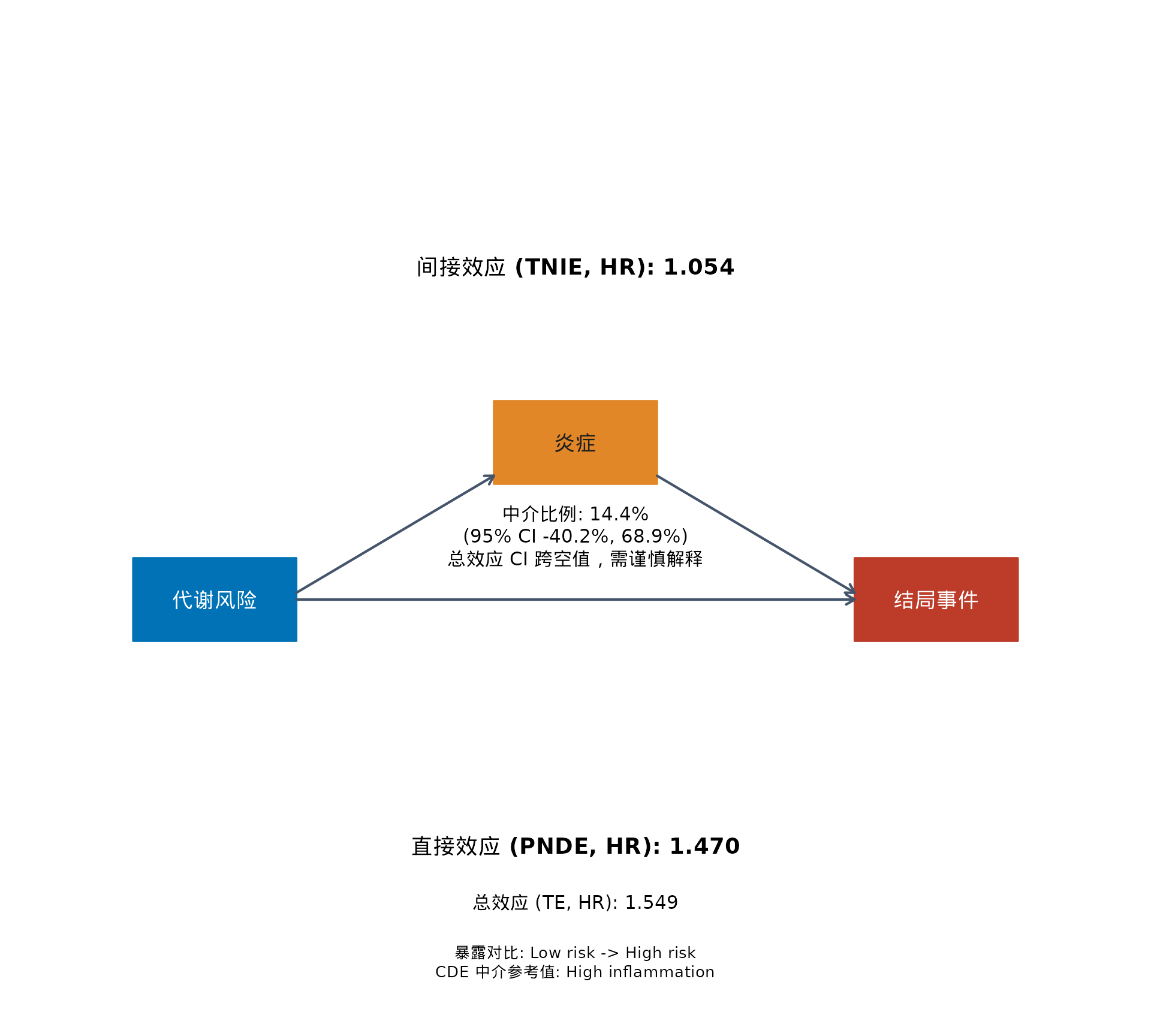
leo_cox_mediation_plot(
  x = res_med,
  model = "Model B",
  exposure_label = "代谢风险",
  mediator_label = "炎症",
  outcome_label = "结局事件",
  language = "zh",
  palette = "jama"
)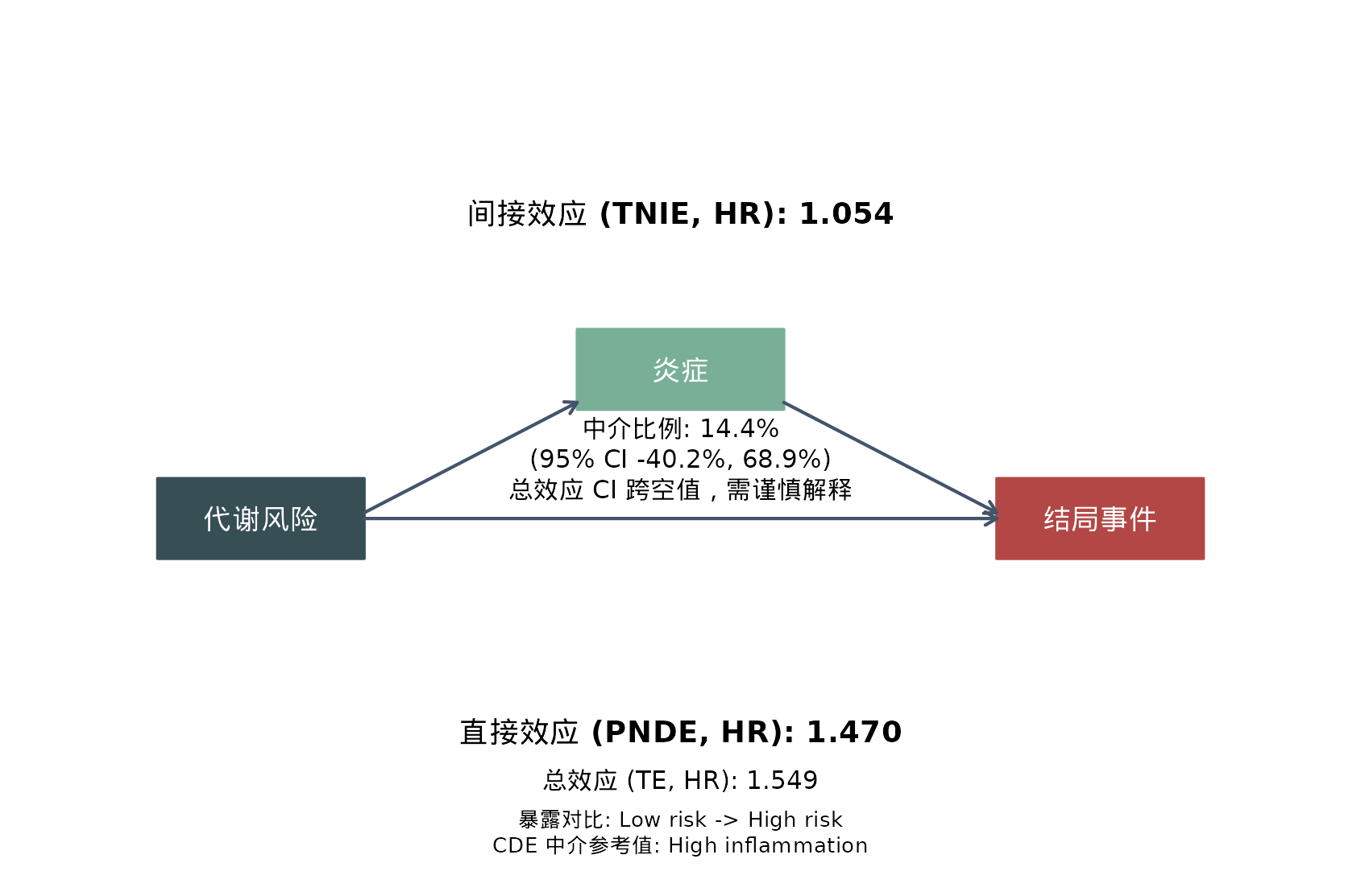
这类图的作用是把最关键的几件事压缩进同一张图里:
- 左边:exposure 对比
- 中间:假定的 mediator
- 右边:incident outcome
- 上方:通过 mediator 的间接路径
- 中间:这条路径大约解释了多少总效应
- 下方:不经过 mediator 的直接路径
还有一个容易误解的点是:这里的间接路径指的是完整的
X -> M -> Y 路径。图里没有把 M -> Y
单独写成一个回归系数,不是因为这部分没建模,而是因为
regmedint 输出的重点是
tnie、pnde、te
这类因果分解量,而不是传统线性中介里的两个路径系数乘积。
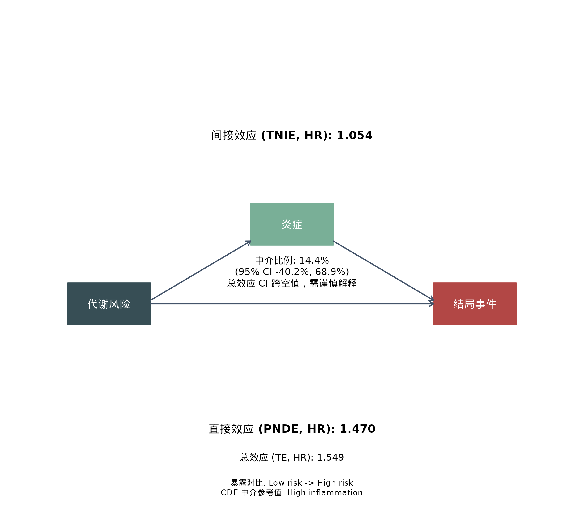
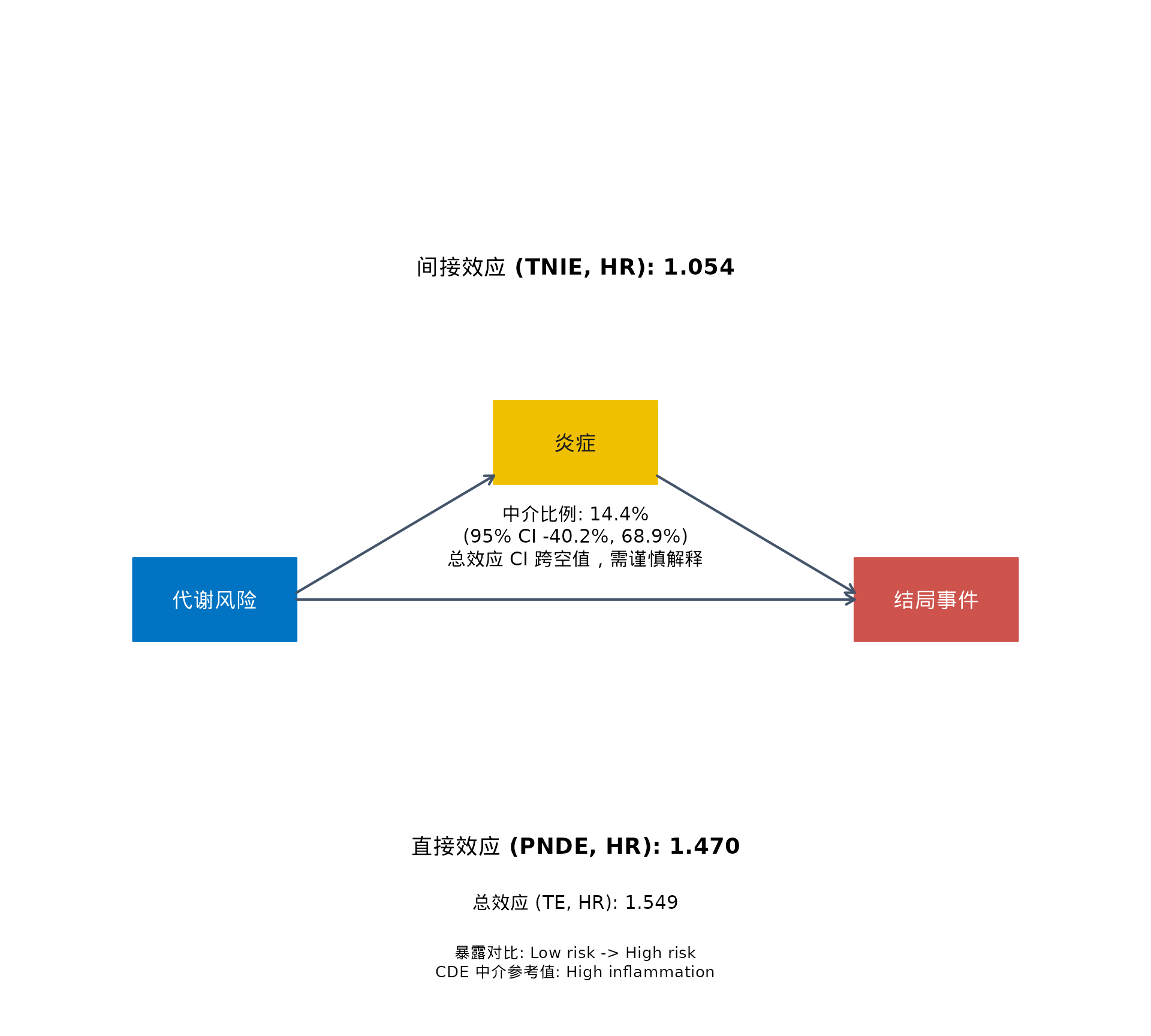
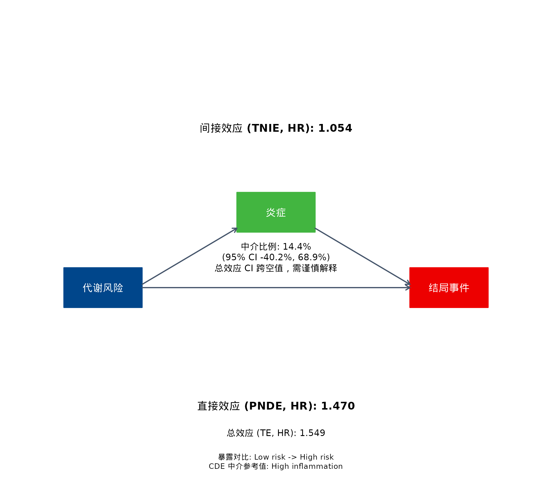
内置期刊风格配色示例
同一套拟合结果,也可以直接切换成几种常见的期刊风格配色。
for (pal in c("jama", "jco", "lancet", "nejm")) {
  leo_cox_mediation_plot(
    x = res_med,
    model = "Model B",
    exposure_label = "代谢风险",
    mediator_label = "炎症",
    outcome_label = "结局事件",
    language = "zh",
    palette = pal
  )
}
Step 3 常见结果模式应该怎么解读
在应用型生存中介分析里,最常见的几种解释模式是:
-
te明显偏离 null,tnie较小,pm为正但不精确:与部分中介一致,但证据还不够强 -
te和tnie都比较清楚,且pm也比较稳定:更支持 mediator 解释了总效应里具有意义的一部分 -
te本身就较弱或跨过 null:pm往往会不稳定,此时更应保守解释 -
yreg自动切换成 AFT:这时除pm外,其他效应量都要按 time ratio 解释,而不是 hazard ratio
所以 Step 3 不只是“跑出一张分解表”,而是要学会什么时候可以讲 pathway,什么时候只能说“结果与某种路径解释一致,但不够精确”。
论文里 Step 3 应该怎么写
比较稳妥的 reporting order 通常是:
- 先报告 main exposure-outcome association
- 再把 mediation 作为 pathway decomposition 的补充证据
- 写清 exposure contrast、mediator reference 和 adjustment profile
- 写清最终用的是哪个
yreg;如果是survCox,说明 rare-event approximation,并直接提醒读者这意味着只有在事件较少时,这个分解更适合作为近似结果报告;如果是 AFT,提醒读者比值尺度应读作 time ratio - 如果 exposure 和 mediator 都来自同一次 baseline visit,直接写明数据本身不能证明 exposure 先于 mediator,把结果写成与假定中介路径一致的分解证据;除非时间顺序有外部支持,否则避免把因果结论写得过强
也就是说,中介分析通常是在主关联已经建立以后,用来细化生物学故事,而不是替代主分析。
本节小结
做完这一步以后,你应该带走 6 个最重要的结论:
- 中介分析讨论的是路径,不是异质性
- 和 Step 1、Step 2 一样,建模前也要先看数据结构和事件负担
-
x_exp_a0、x_exp_a1、x_med_cde、x_cov_cond决定了中介效应在哪里被评价 -
mreg控制x_med ~ x_exp + x_cov,yreg控制time ~ x_exp + x_med + x_cov,interaction = TRUE会在 outcome 模型里加入x_exp:x_med -
yreg = "auto"会在事件率<= 10%时选survCox(也就意味着后续分解依赖 rare-event approximation,也就是只有在事件较少时才更适合作为近似分解来理解),否则选survAFT_weibull - factor mediator 不应该强行塞进
mreg = "linear",最终结果也必须结合实际 outcome model、不确定性和时间顺序一起解释