Visualize continuous effect values (e.g., log2FC/beta/FC) across groups with a reference dashed line. Non-significant points (by p-value and/or deadband) are drawn in gray; significant points use a diverging palette.
Usage
plot_dbee(
  df,
  group.by,
  effect_col,
  p_col = NULL,
  p_thresh = 0.05,
  effect_thresh = 0,
  pal_color = c(low = "#5062A7", mid = "white", high = "#BC4B59"),
  log2fc_limits = NULL,
  insignificant_color = "gray80",
  deadband = NULL,
  flip_coord = TRUE,
  point_size = 1,
  seed = NULL,
  ...
)
Arguments
- df
data.frame/tibble containing grouping and effect columns
- group.by
character, column name for grouping
- effect_col
character, column name for effect (e.g., "logFC", "beta")
- p_col
character or NULL, column name for p-values; if provided, p >= p_thresh is treated as non-significant
- p_thresh
numeric, p-value threshold for significance (default 0.05)
- effect_thresh
numeric, reference threshold for dashed line and color midpoint (default 0)
- pal_color
named vector c(low, mid, high) for diverging palette (default c(low="#5062A7", mid="white", high="#BC4B59"))
- log2fc_limits
NULL or numeric length-2 c(L, R); if set, color scale limits are c(effect_thresh-L, effect_thresh+R)
- insignificant_color
character, color for non-significant/gray-zone points (default "gray80")
- deadband
NULL or non-negative numeric; if set, |effect - effect_thresh| <= deadband will be gray
- flip_coord
logical, flip coordinates to show groups vertically (default TRUE)
- point_size
numeric, point size (default 1)
- seed
NULL or integer, for reproducible quasirandom placement
- ...
extra args passed to ggbeeswarm::geom_quasirandom()
Examples
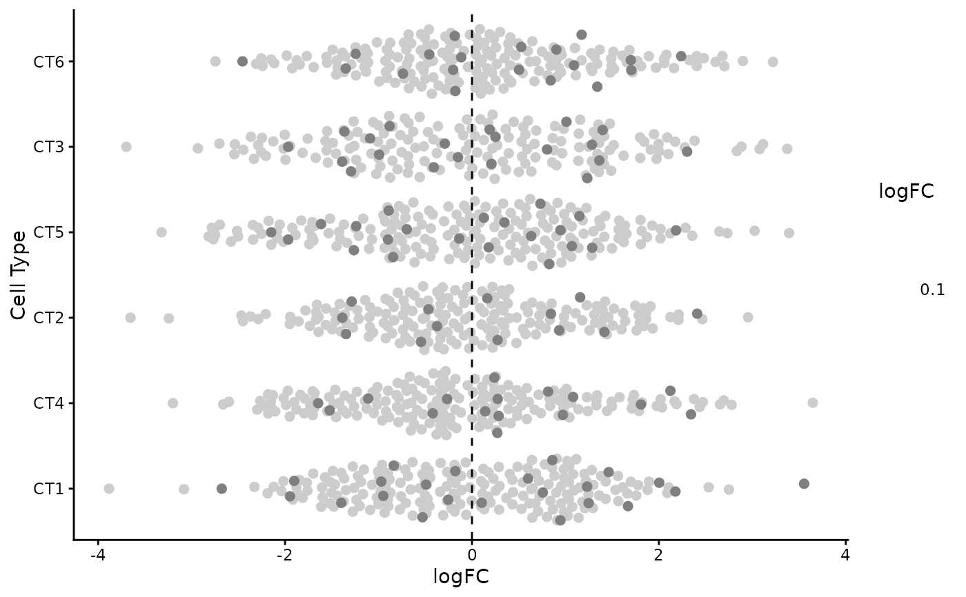
# ---- Example 1: MiloR-like DA results ----
set.seed(1)
milo_df <- tibble::tibble(
Nhood = paste0("n", seq_len(1200)),
`Cell Type` = sample(paste0("CT", 1:6), 1200, replace = TRUE),
logFC = rnorm(1200, sd = 1.2),
SpatialFDR = runif(1200)
)
# Visualize logFC by cell types; non-sig: SpatialFDR >= 0.1; dashed line at 0
p1 <- plot_dbee(milo_df, group.by = "Cell Type", effect_col = "logFC",
p_col = "SpatialFDR", p_thresh = 0.1, effect_thresh = 0,
log2fc_limits = c(-.1, .1), deadband = 0.1, point_size = 2, seed = 42)
#> ℹ [05:06:05] plot_dbee(): start; rows=1200, groups=6
#> ✔ [05:06:05] plot_dbee(): done
print(p1)
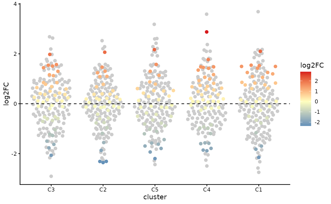
 # ---- Example 2: scRNA-seq DEG-like results ----
set.seed(123)
deg_df <- tibble::tibble(
gene = paste0("G", 1:900),
cluster = sample(paste0("C", 1:5), 900, replace = TRUE),
log2FC = rnorm(900, mean = rep(seq(-0.4, 0.4, length.out = 5), each = 180), sd = 1),
p_val_adj = pmin(runif(900)^2, 1)
)
# Visualize log2FC by cluster
p2 <- plot_dbee(
deg_df, group.by = "cluster",
effect_col = "log2FC",
p_col = "p_val_adj", p_thresh = 0.05,
effect_thresh = 0,
pal_color = c(
low = "#2C7BB6", mid = "#FFFFBF",
high = "#D7191C"),
flip_coord = FALSE,
log2fc_limits = NULL, deadband = 0.05,
point_size = 2, seed = 7)
#> ℹ [05:06:05] plot_dbee(): start; rows=900, groups=5
#> ✔ [05:06:05] plot_dbee(): done
print(p2)
# ---- Example 2: scRNA-seq DEG-like results ----
set.seed(123)
deg_df <- tibble::tibble(
gene = paste0("G", 1:900),
cluster = sample(paste0("C", 1:5), 900, replace = TRUE),
log2FC = rnorm(900, mean = rep(seq(-0.4, 0.4, length.out = 5), each = 180), sd = 1),
p_val_adj = pmin(runif(900)^2, 1)
)
# Visualize log2FC by cluster
p2 <- plot_dbee(
deg_df, group.by = "cluster",
effect_col = "log2FC",
p_col = "p_val_adj", p_thresh = 0.05,
effect_thresh = 0,
pal_color = c(
low = "#2C7BB6", mid = "#FFFFBF",
high = "#D7191C"),
flip_coord = FALSE,
log2fc_limits = NULL, deadband = 0.05,
point_size = 2, seed = 7)
#> ℹ [05:06:05] plot_dbee(): start; rows=900, groups=5
#> ✔ [05:06:05] plot_dbee(): done
print(p2)