Overview
This tutorial demonstrates the Functional Inference Pipeline
(FIP) via silico_ko() from
leo.sc.
FIP estimates gene-associated transcriptional programs by comparing
cells with low versus high endogenous
expression of a target gene g, conceptually
mimicking transcriptional changes after a perturbation knock-down — but
entirely in silico using existing single-cell data. The
function is named silico_ko() (SKO) for memorability, but
the underlying logic is more akin to endogenous knock-down /
over-expression contrasting rather than a true genetic
knockout.
-
Dataset:
SeuratObject::pbmc_small(80-cell Seurat demo object, for illustration only) - Goal: Identify functional gene programs associated with the perturbation of a target gene
- Output: Cell-type composition of high-expressors, DEG table, and enrichment results
Method
FIP proceeds in six steps:
-
Filter: Exclude cells with zero target-gene
expression; remove rare cell types (<
filter_cell_thresholdcells). - Rank: Rank all remaining g-expressing cells (N) by expression of the target gene.
-
Select ghigh: Select the top
cells (top
pct_thresholdfraction, e.g., 0.1 = 10%; orabs_thresholdabsolute count) as the high-expression group, preserving cell-type composition. - Match glow: Select an equal number of bottom cells as the low-expression group with matched cell-type composition to minimise lineage confounding.
-
DEG: Apply
Seurat::FindMarkers()(Wilcoxon rank-sum; glow asident.1) to identify differentially expressed genes between groups. -
Enrichment: Run
leo.basic::leo_enrich()(ORA / GSEA against GO, KEGG, or custom backgrounds) to infer the biological functions associated with ghigh vs glow.
Data & Gene Setup
data("pbmc_small", package = "SeuratObject")
srt <- pbmc_small

# Annotate clusters with broad cell-type labels
# Source: https://satijalab.org/seurat/articles/pbmc3k_tutorial
srt$cell_anno <- dplyr::recode(
  as.character(Seurat::Idents(srt)),
  "0" = "T/NK cells", "1" = "CD14+ Monocytes", "2" = "B cells"
)

# Pick a target gene: here we choose NKG7 for illustration.
gene_use <- "NKG7"
gene_use
#> [1] "NKG7"
⚠️ Method accuracy note:
pbmc_smallcontains only 80 cells and is used here purely for a reproducible demo. DEG and enrichment results are statistically underpowered and should not be interpreted biologically. For a realistic FIP result, see the real-world example below.
Run SKO
res <- silico_ko(
  all = srt,
  gene = gene_use,
  sko_mode = "ko",
  cell_col = "cell_anno",
  filter_cell_threshold = 3,
  pct_threshold = 0.2,
  deg_method = "default",
  enrichment_method = "ORA",
  enrichment_bg = "GO",
  simplify = FALSE # pbmc_small is too small for reliable simplification
)
#> ℹ [05:06:42] Performing in-silico knock-down for: NKG7
#> ℹ Step 1: Filtering cells expressing the target gene.
#> ! [05:06:42] Only 35 cells express NKG7, results may be unstable.
#> ℹ [05:06:42] Found 35 cells expressing NKG7.
#> ℹ Found 3 cell type(s) with > 3 cells. Applying filter...
#> ℹ [05:06:42] After subset cell_anno for **B cells, CD14+ Monocytes, and T/NK cells**, 35 cells remains.
#> ! [05:06:42] n_extract < 100, set to 100 to ensure minimal power.
#> ℹ Step 2: Extracting top 100 cells with high NKG7 expression.
#> ℹ Calculating quota for each cell type based on 50% of expressing cells.
#> ! [05:06:42] Requested 100 exceeds per-type 50% cap (max 17). Resetting to 17.
#> ℹ [05:06:42] High group composition (N = 17): T/NK cells: 8 (47.1%), CD14+ Monocytes: 5 (29.4%), B cells: 4 (23.5%)
#> ℹ Step 4: Locating bottom 17 matched cells.
#> ℹ Step 5: Performing differential expression analysis (default).
#> ℹ [05:06:42] After subset sko_group for **high and low**, 34 cells remains.
#> For a (much!) faster implementation of the Wilcoxon Rank Sum Test,
#> (default method for FindMarkers) please install the presto package
#> --------------------------------------------
#> install.packages('devtools')
#> devtools::install_github('immunogenomics/presto')
#> --------------------------------------------
#> After installation of presto, Seurat will automatically use the more
#> efficient implementation (no further action necessary).
#> This message will be shown once per session
#> ℹ [05:06:42] DEG done --> more expressed in [low]: 0; more expressed in [high]: 0
#> ℹ Step 6: Performing enrichment analysis.
#> ℹ [05:06:42] A total of 1 methods and  1 backgrounds  (1 round) enrichment will be processed.
#> ℹ [05:06:42] Round 1: Processing ORA for GO background...
#>
#>
#> ✔ [05:07:32] FIP completed successfully.
#> ✔ [05:07:32] Elapsed 50.03 sec

names(res)
#> [1] "high_cells"  "low_cells"   "cell_rato"   "deg_results" "enrichments"
Interpret Outputs
length(res$high_cells)
#> [1] 17
length(res$low_cells)
#> [1] 17

head(res$cell_rato)
#> # A tibble: 3 × 3
#>   cell_type           n   pct
#>   <chr>           <int> <dbl>
#> 1 T/NK cells          8  47.1
#> 2 CD14+ Monocytes     5  29.4
#> 3 B cells             4  23.5

deg <- res$deg_results
deg <- tibble::rownames_to_column(deg, "gene")
head(deg[, c("gene", "avg_log2FC", "p_val_adj")])
#>     gene avg_log2FC p_val_adj
#> 1   NKG7  -1.790060 0.2771519
#> 2   GZMB  -2.122172 1.0000000
#> 3   TCF7   9.377081 1.0000000
#> 4   PRF1  -2.389099 1.0000000
#> 5  SNHG7   8.081088 1.0000000
#> 6 MS4A6A   7.546991 1.0000000

if (length(res$enrichments) == 0) {
  cat("No enrichment result was returned (expected for very small demo data).\n")
} else {
  print(names(res$enrichments))
}
#> No enrichment result was returned (expected for very small demo data).
Caveats
-
pbmc_smallis intentionally tiny and is only used here to keep the demo lightweight. - Enrichment output can be empty (
res$enrichmentsmay belist()) and this is expected in small datasets. - For biological interpretation, use larger datasets and review
parameters such as
pct_threshold,filter_cell_threshold, and the enrichment background.
Real-World Example: LRRK2 in VKH Disease
To demonstrate FIP’s capability to uncover biological insights at
scale, we now walk through a real-world result from a
Vogt–Koyanagi–Harada (VKH) disease study, in which
silico_ko() was applied to LRRK2 across a
scRNA-seq cohort of 34 VKH patients and 14 healthy controls.
Load pre-computed FIP result
The pre-computed result is hosted on GitHub Releases. We download it once and cache it locally:
data_url <- "https://github.com/laleoarrow/leo.sc/releases/download/data-v2/LRRK2_ko_res.rds"
cache_dir <- tools::R_user_dir("leo.sc", which = "cache")
if (!dir.exists(cache_dir)) dir.create(cache_dir, recursive = TRUE)
dest <- file.path(cache_dir, "LRRK2_ko_res.rds")
if (!file.exists(dest)) {
  message("Downloading LRRK2 FIP result (7.8 MB) ...")
  utils::download.file(data_url, dest, mode = "wb", quiet = TRUE)
}
#> Downloading LRRK2 FIP result (7.8 MB) ...

lrrk2 <- readRDS(dest) # **This represents a standard output object generated by FIP.**
names(lrrk2)
#> [1] "high_cells"  "low_cells"   "cell_rato"   "deg_results" "enrichments"
Understanding the comparison direction
In FIP’s KO mode, ident.1 = "low"
(simulated knock-out) and ident.2 = "high"
(wild-type–like). According to Seurat::FindMarkers()
convention:
-
avg_log2FC > 0→ gene is up-regulated after simulated KO (more expressed in glow) -
avg_log2FC < 0→ gene is down-regulated after simulated KO (more expressed in ghigh)
Cell-type composition of ghigh
FIP preserves cell-type composition between ghigh and glow groups, ensuring that DEGs reflect variation in LRRK2 expression within each lineage as a whole rather than confounding by certain cell-type abundance:
# Number of high- and low-expression cells
cat("g_high cells:", length(lrrk2$high_cells), "\n")
#> g_high cells: 1937
cat("g_low  cells:", length(lrrk2$low_cells), "\n")
#> g_low  cells: 1937

# Cell-type composition of the high-expression group
knitr::kable(
  head(lrrk2$cell_rato, 10),
  caption = "Top 10 cell types in LRRK2-high group (pct = percentage)"
)| cell_type | n | pct |
|---|---|---|
| Classic Monocyte_PRKAG2 | 539 | 27.8 |
| Classic Monocyte_S100A12 | 501 | 25.9 |
| B_c1_Naïve_IGHD | 249 | 12.9 |
| B_c0_Memory_TNFRSF13B | 214 | 11.0 |
| Non-classic Monocyte | 183 | 9.4 |
| moDC | 106 | 5.5 |
| CD1C cDC | 27 | 1.4 |
| CD4_c3_Th17_RORA | 13 | 0.7 |
| CD8_c0_TEMRA_FGFBP2 | 10 | 0.5 |
| CD8_c1_Tem_ZEB2 | 9 | 0.5 |
Differential expression summary
deg <- lrrk2$deg_results
up <- sum(deg$avg_log2FC > 0 & deg$p_val_adj < 0.05)
down <- sum(deg$avg_log2FC < 0 & deg$p_val_adj < 0.05)
cat("Significant DEGs (FDR < 0.05):\n")
#> Significant DEGs (FDR < 0.05):
cat("  Up after KO (log2FC > 0):  ", up, "\n")
#>   Up after KO (log2FC > 0):   2826
cat("  Down after KO (log2FC < 0):", down, "\n")
#>   Down after KO (log2FC < 0): 5459

# Top 10 genes up-regulated after simulated KO
deg_df <- tibble::rownames_to_column(deg, "gene")
top_up <- head(deg_df[deg_df$avg_log2FC > 0 & deg_df$p_val_adj < 0.05, ], 10)
knitr::kable(
  top_up[, c("gene", "avg_log2FC", "p_val_adj")],
  digits = 3,
  caption = "Top 10 genes up-regulated after simulated LRRK2 knock-out"
)| gene | avg_log2FC | p_val_adj | |
|---|---|---|---|
| 2 | COX8A | 1.261 | 0 |
| 3 | COX6A1 | 1.292 | 0 |
| 4 | PFN1 | 1.212 | 0 |
| 5 | SLC35F1 | 1.355 | 0 |
| 6 | OST4 | 1.053 | 0 |
| 7 | RBFOX2 | 1.208 | 0 |
| 8 | S100A11 | 1.502 | 0 |
| 9 | MIF | 1.131 | 0 |
| 10 | CSTB | 1.356 | 0 |
| 11 | GNG5 | 1.103 | 0 |
GSEA enrichment (GO)
The enrichment results are stored in
lrrk2$enrichments:
cat("Available enrichment results:\n")
#> Available enrichment results:
print(names(lrrk2$enrichments))
#> [1] "GSEA_GO"       "GSEA_KEGG"     "GSEA_Reactome"
Three representative GO pathways are visualised below using
enrichplot::gseaplot2():
library(enrichplot)
#> enrichplot v1.30.5 Learn more at https://yulab-smu.top/contribution-knowledge-mining/
#>
#> Please cite:
#>
#> Guangchuang Yu, Li-Gen Wang, Guang-Rong Yan, Qing-Yu He. DOSE: an
#> R/Bioconductor package for Disease Ontology Semantic and Enrichment
#> analysis. Bioinformatics. 2015, 31(4):608-609
gseaplot2(
  lrrk2$enrichments$GSEA_GO,
  color = ggsci::pal_npg("nrc")(3),
  geneSetID = c("GO:0003823", "GO:0006119", "GO:0001909"),
  subplots = 1:2,
  pvalue_table = TRUE
)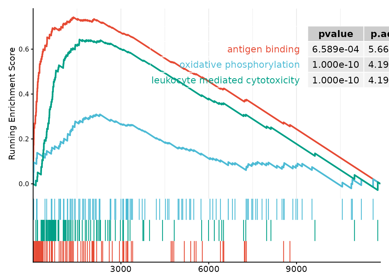
GSEA enrichment plot for LRRK2-high vs LRRK2-low contrast (GO). Top enriched pathways: antigen binding, oxidative phosphorylation, and leukocyte-mediated cytotoxicity.
Key biological insight.: All three pathways show positive NES, meaning they are up-regulated in the LRRK2-low (simulated KO) group. This implies that LRRK2 normally suppresses these immune programmes under physiological conditions. Notably, this computational prediction aligns with experimental evidence: Gardet et al. demonstrated that LRRK2 controls inflammatory cytokine production via NF-κB phosphorylation and antigen presentation in bone marrow-derived dendritic cells (Int J Mol Sci 2020;21:6097). The concordance between FIP’s in silico inference and wet-lab perturbation underscores the method’s utility for generating testable hypotheses from single-cell data.